如何用 WebGL 绘制 3D 物体
# 如何用 WebGL 绘制 3D 物体
# 如何用 WebGL 绘制三维立方体
首先,我们来绘制熟悉的 2D 图形,比如矩形,再把它拓展到三维空间变成立方体。
// vertex shader 顶点着色器
attribute vec2 a_vertexPosition;
attribute vec4 color;

varying vec4 vColor;

void main() {
  gl_PointSize = 1.0;
  vColor = color;
  gl_Position = vec4(a_vertexPosition, 1, 1);
}
2
3
4
5
6
7
8
9
10
11
// fragment shader 片元着色器
#ifdef GL_ES
precision highp float;
#endif

varying vec4 vColor;

void main() {
  gl_FragColor = vColor;
}
2
3
4
5
6
7
8
9
10
// ...
// 顶点信息
renderer.setMeshData([{
  positions: [
    [-0.5, -0.5],
    [-0.5, 0.5],
    [0.5, 0.5],
    [0.5, -0.5],
  ],
  attributes: {
    color: [
      [1, 0, 0, 1],
      [1, 0, 0, 1],
      [1, 0, 0, 1],
      [1, 0, 0, 1],
    ],
  },
  cells: [[0, 1, 2], [0, 2, 3]],
}]);
renderer.render();
2
3
4
5
6
7
8
9
10
11
12
13
14
15
16
17
18
19
20
通过这几段代码,就在画布上绘制出了一个红色的矩形。
接下来,要想把 2 维矩形拓展到 3 维,我们的第一步就是要把顶点扩展到 3 维。这一步的操作比较简单,我们只需要把顶点从 vec2 扩展到 vec3 就可以了。
// vertex shader
attribute vec3 a_vertexPosition;
attribute vec4 color;

varying vec4 vColor;

void main() {
  gl_PointSize = 1.0;
  vColor = color;
  gl_Position = vec4(a_vertexPosition, 1);
}
2
3
4
5
6
7
8
9
10
11
然后,我们需要计算立方体的顶点数据。一个立方体有 8 个顶点,这 8 个顶点能组成 6 个面。在 WebGL 中,我们就需要用 12 个三角形来绘制它。如果每个面的属性相同,我们就可以复用 8 个顶点来绘制。而如果属性不同,比如每个面要绘制成不同的颜色,或者添加不同的纹理图片,我们还得把每个面的顶点分开。这样的话,我们一共需要 24 个顶点。

为了方便使用,可以写一个 JavaScript 函数,用来生成立方体 6 个面的 24 个顶点,以及 12 个三角形的索引,并且直接在这个函数里定义了每个面的颜色。
function cube(size = 1.0, colors = [[1, 0, 0, 1]]) {
  const h = 0.5 * size;
  const vertices = [
    [-h, -h, -h],
    [-h, h, -h],
    [h, h, -h],
    [h, -h, -h],
    [-h, -h, h],
    [-h, h, h],
    [h, h, h],
    [h, -h, h],
  ];

  const positions = [];
  const color = [];
  const cells = [];

  let colorIdx = 0;
  let cellsIdx = 0;
  const colorLen = colors.length;

  function quad(a, b, c, d) {
    [a, b, c, d].forEach((i) => {
      positions.push(vertices[i]);
      color.push(colors[colorIdx % colorLen]);
    });
    cells.push(
      [0, 1, 2].map(i => i + cellsIdx),
      [0, 2, 3].map(i => i + cellsIdx),
    );
    colorIdx++;
    cellsIdx += 4;
  }

  quad(1, 0, 3, 2);
  quad(4, 5, 6, 7);
  quad(2, 3, 7, 6);
  quad(5, 4, 0, 1);
  quad(3, 0, 4, 7);
  quad(6, 5, 1, 2);

  return {positions, color, cells};
}
2
3
4
5
6
7
8
9
10
11
12
13
14
15
16
17
18
19
20
21
22
23
24
25
26
27
28
29
30
31
32
33
34
35
36
37
38
39
40
41
42
43
这样,我们就可以构建出立方体的顶点信息。下面是立方体的 12 个顶点。
const geometry = cube(1.0, [
  [1, 0, 0, 1],
  [0, 0.5, 0, 1],
  [1, 0, 1, 1],
]);
2
3
4
5
通过上面的代码,我们就能创建出一个棱长为 1 的立方体,并且六个面的颜色分别是 “红、绿、蓝、红、绿、蓝”。
# 深度检测和深度缓冲区
绘制 3D 图形与绘制 2D 图形有一点不一样,那就是我们必须要开启深度检测和启用深度缓冲区。在 WebGL 中,我们可以通过 gl.enable(gl.DEPTH_TEST) 来开启深度检测。
而且,我们在清空画布的时候,也要用 gl.clear(gl.COLOR_BUFFER_BIT | gl.DEPTH_BUFFER_BIT); 来同时清空颜色缓冲区和深度缓冲区。启动和清空深度检测和深度缓冲区这两个步骤,是这个过程中非常重要的一环,但是我们几乎不会用原生的方式来写代码,所以我们了解到这个程度就可以了。
这些步骤可以直接使用 gl-renderer (opens new window) 库,它封装了深度检测,在使用它的时候,我们只要在创建 renderer 的时候设置一个参数 depth: true 即可。
下面就用 gl-renderer 将这个三维立方体渲染出来。
const canvas = document.querySelector('canvas');
const renderer = new GlRenderer(canvas, {
  depth: true,
});

const program = renderer.compileSync(fragment, vertex);
renderer.useProgram(program);

renderer.setMeshData([{
  positions: geometry.positions,
  attributes: {
    color: geometry.color,
  },
  cells: geometry.cells,
}]);
renderer.render();
2
3
4
5
6
7
8
9
10
11
12
13
14
15
16
不过,执行完代码后会发现,我们只能看到立方体的一个红色的面。
# 投影矩阵:变换 WebGL 坐标系
重新看下刚刚的代码,会发现:
立方体的顶点是这么定义的:
const vertices = [
  [-h, -h, -h],
  [-h, h, -h],
  [h, h, -h],
  [h, -h, -h],
  [-h, -h, h],
  [-h, h, h],
  [h, h, h],
  [h, -h, h],
]
2
3
4
5
6
7
8
9
10
而立方体的六个面的颜色是这么定义的:
// 立方体的六个面
quad(1, 0, 3, 2); // 红 -- 这一面应该朝内
quad(4, 5, 6, 7); // 绿 -- 这一面应该朝外
quad(2, 3, 7, 6); // 蓝
quad(5, 4, 0, 1); // 红
quad(3, 0, 4, 7); // 绿
quad(6, 5, 1, 2); // 蓝
2
3
4
5
6
7
这里有个问题,WebGL 的坐标系是 z 轴向外为正,z 轴向内为负,所以根据我们的代码,赋给靠外那一面的颜色应该是绿色,而不是红色。但是这个立方体朝向我们的一面却是红色。
实际上,WebGL 默认的剪裁坐标的 z 轴方向,的确是朝内的。也就是说,WebGL 坐标系就是一个左手系而不是右手系。但是,基本上所有的 WebGL 教程,也包括我们前面的课程,一直都在说 WebGL 坐标系是右手系,这又是为什么呢?
这是因为,规范的直角坐标系是右手坐标系,符合我们的使用习惯。因此,一般来说,不管什么图形库或图形框架,在绘图的时候,都会默认将坐标系从左手系转换为右手系。
因此,下一步就是要将 WebGL 的坐标系从左手系转换为右手系。关于坐标转换,我们可以通过齐次矩阵来完成。将左手系坐标转换为右手系,实际上就是将 z 轴坐标方向反转,对应的齐次矩阵如下:
[
  1, 0, 0, 0,
  0, 1, 0, 0,
  0, 0, -1, 0,
  0, 0, 0, 1
]
2
3
4
5
6
这种转换坐标的齐次矩阵,又被称为投影矩阵(ProjectionMatrix)。投影矩阵不仅可以用来改变 z 轴坐标,还可以用来实现正交投影、透视投影以及其他的投影变换。
接着,将投影矩阵加入到顶点着色器中,画布上显示的就是绿色的正方形了。
attribute vec3 a_vertexPosition;
attribute vec4 color;

varying vec4 vColor;
uniform mat4 projectionMatrix;

void main() {
  gl_PointSize = 1.0;
  vColor = color;
  gl_Position = projectionMatrix * vec4(a_vertexPosition, 1.0);
}
2
3
4
5
6
7
8
9
10
11
# 模型矩阵:让立方体旋转起来
经过投影矩阵转换之后,我们还是只能看到立方体的一个面,因为我们的视线正好是垂直于 z 轴的,所以其他的面被完全挡住了。不过,我们可以通过旋转立方体,将其他的面露出来。旋转立方体,同样可以通过矩阵运算来实现。
这次我们要用到另一个齐次矩阵,它定义了被绘制的物体变换,这个矩阵叫做模型矩阵(ModelMatrix)。接下来,我们就把模型矩阵加入到顶点着色器中,然后将它与投影矩阵相乘,最后再乘上齐次坐标,就得到最终的顶点坐标了。
attribute vec3 a_vertexPosition;
attribute vec4 color;

varying vec4 vColor;
uniform mat4 projectionMatrix;
uniform mat4 modelMatrix;

void main() {
  gl_PointSize = 1.0;
  vColor = color;
  gl_Position = projectionMatrix * modelMatrix * vec4(a_vertexPosition, 1.0);
}
2
3
4
5
6
7
8
9
10
11
12
接着,我们定义一个 JavaScript 函数,用立方体沿 x、y、z 轴的旋转来生成模型矩阵。我们以 x、y、z 三个方向的旋转得到三个齐次矩阵,然后将它们相乘,就能得到最终的模型矩阵。
import {multiply} from '../common/lib/math/functions/Mat4Func.js';

function fromRotation(rotationX, rotationY, rotationZ) {
  let c = Math.cos(rotationX);
  let s = Math.sin(rotationX);
  const rx = [
    1, 0, 0, 0,
    0, c, s, 0,
    0, -s, c, 0,
    0, 0, 0, 1,
  ];

  c = Math.cos(rotationY);
  s = Math.sin(rotationY);
  const ry = [
    c, 0, s, 0,
    0, 1, 0, 0,
    -s, 0, c, 0,
    0, 0, 0, 1,
  ];

  c = Math.cos(rotationZ);
  s = Math.sin(rotationZ);
  const rz = [
    c, s, 0, 0,
    -s, c, 0, 0,
    0, 0, 1, 0,
    0, 0, 0, 1,
  ];

  const ret = [];
  multiply(ret, rx, ry);
  multiply(ret, ret, rz);
  return ret;
}
2
3
4
5
6
7
8
9
10
11
12
13
14
15
16
17
18
19
20
21
22
23
24
25
26
27
28
29
30
31
32
33
34
35
最后,我们把这个模型矩阵传给顶点着色器,不断更新三个旋转角度,就能实现立方体旋转的效果,也就可以看到立方体其他各个面了。最终效果看这里 (opens new window)。
let rotationX = 0;
let rotationY = 0;
let rotationZ = 0;

function update() {
  rotationX += 0.003;
  rotationY += 0.005;
  rotationZ += 0.007;
  renderer.uniforms.modelMatrix = fromRotation(rotationX, rotationY, rotationZ);
  requestAnimationFrame(update);
}
update();
2
3
4
5
6
7
8
9
10
11
12
# 如何用 WebGL 绘制圆柱体
除了绘制立方体,我们还可以构建顶点和三角形,来绘制更加复杂的图形,比如圆柱体、球体等等。
圆柱体的两个底面都是圆,我们可以用割圆的方式对圆进行简单的三角剖分,然后把圆柱的侧面用上下两个圆上的顶点进行三角剖分。
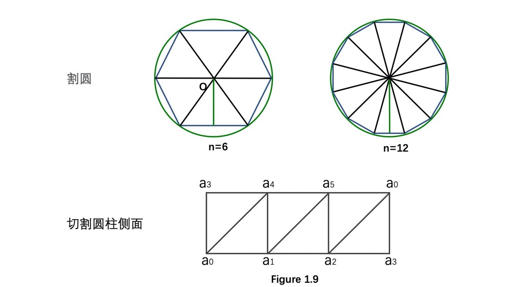
具体算法如下:
function cylinder(radius = 1.0, height = 1.0, segments = 30, colorCap = [0, 0, 1, 1], colorSide = [1, 0, 0, 1]) {
  const positions = [];
  const cells = [];
  const color = [];
  const cap = [[0, 0]];
  const h = 0.5 * height;

  // 顶和底的圆
  for(let i = 0; i <= segments; i++) {
    const theta = Math.PI * 2 * i / segments;
    const p = [radius * Math.cos(theta), radius * Math.sin(theta)];
    cap.push(p);
  }

  positions.push(...cap.map(([x, y]) => [x, y, -h]));
  for(let i = 1; i < cap.length - 1; i++) {
    cells.push([0, i, i + 1]);
  }
  cells.push([0, cap.length - 1, 1]);

  let offset = positions.length;
  positions.push(...cap.map(([x, y]) => [x, y, h]));
  for(let i = 1; i < cap.length - 1; i++) {
    cells.push([offset, offset + i, offset + i + 1]);
  }
  cells.push([offset, offset + cap.length - 1, offset + 1]);

  color.push(...positions.map(() => colorCap));

  // 侧面
  offset = positions.length;
  for(let i = 1; i < cap.length; i++) {
    const a = [...cap[i], h];
    const b = [...cap[i], -h];
    const nextIdx = i < cap.length - 1 ? i + 1 : 1;
    const c = [...cap[nextIdx], -h];
    const d = [...cap[nextIdx], h];

    positions.push(a, b, c, d);
    color.push(colorSide, colorSide, colorSide, colorSide);
    cells.push([offset, offset + 1, offset + 2], [offset, offset + 2, offset + 3]);
    offset += 4;
  }

  return {positions, cells, color};
}
2
3
4
5
6
7
8
9
10
11
12
13
14
15
16
17
18
19
20
21
22
23
24
25
26
27
28
29
30
31
32
33
34
35
36
37
38
39
40
41
42
43
44
45
46
把前面立方体的代码里的 cube 改为 cylinder,就可以绘制出圆柱体了。
总的来说,用 WebGL 绘制三维物体,实际上和绘制二维物体没有什么本质不同,都是将图形(对于三维来说,也就是几何体)的顶点数据构造出来,然后将它们送到缓冲区中,再执行绘制。只不过三维图形的绘制需要构造三维的顶点和网格,在绘制前还需要启用深度缓冲区。
# 构造和使用法向量:实现光照效果
在前面的例子中,我们构造出了几何体的顶点信息,包括顶点的位置和颜色信息,除此之外,我们还可以构造几何体的其他信息,其中一种比较有用的信息是顶点的法向量信息。
法向量表示每个顶点所在的面的法线方向,法向量非常有用,在 3D 渲染中,我们可以通过法向量来计算光照、阴影、进行边缘检测等等。
# 1. 构造法向量
对于立方体来说,得到法向量非常简单,我们只要找到垂直于立方体 6 个面上的线段,再得到这些线段所在向量上的单位向量就行了。
[0, 0, -1]
[0, 0, 1]
[0, -1, 0]
[0, 1, 0]
[-1, 0, 0]
[1, 0, 0]
2
3
4
5
6
对于圆柱体来说,底面和顶面法线分别是 (0, 0, -1) 和 (0, 0, 1)。侧面的计算稍微复杂一些,需要通过三角网格来计算。
因为几何体是由三角网格构成的,而法线是垂直于三角网格的线,如果要计算法线,我们可以借助三角形的顶点,使用向量的叉积定理 (opens new window)来求。我们假设在一个平面内,有向量 a 和 b,n 是它们的法向量,那我们可以得到公式:n = a X b。
根据这个公式,我们可以通过以下方法求出侧面的法向量:
const tmp1 = [];
const tmp2 = [];
// 侧面
offset = positions.length;
for (let i = 1; i < cap.length; i++) {
  const a = [...cap[i], h];
  const b = [...cap[i], -h];
  const nextIdx = i < cap.length - 1 ? i + 1 : 1;
  const c = [...cap[nextIdx], -h];
  const d = [...cap[nextIdx], h];

  positions.push(a, b, c, d);

  const norm = [];
  cross(norm, subtract(tmp1, b, a), subtract(tmp2, c, a));
  normalize(norm, norm);
  normal.push(norm, norm, norm, norm); // abcd 四个点共面,它们的法向量相同
  color.push(colorSide, colorSide, colorSide, colorSide);
  cells.push([offset, offset + 1, offset + 2], [offset, offset + 2, offset + 3]);
  offset += 4;
}
2
3
4
5
6
7
8
9
10
11
12
13
14
15
16
17
18
19
20
21
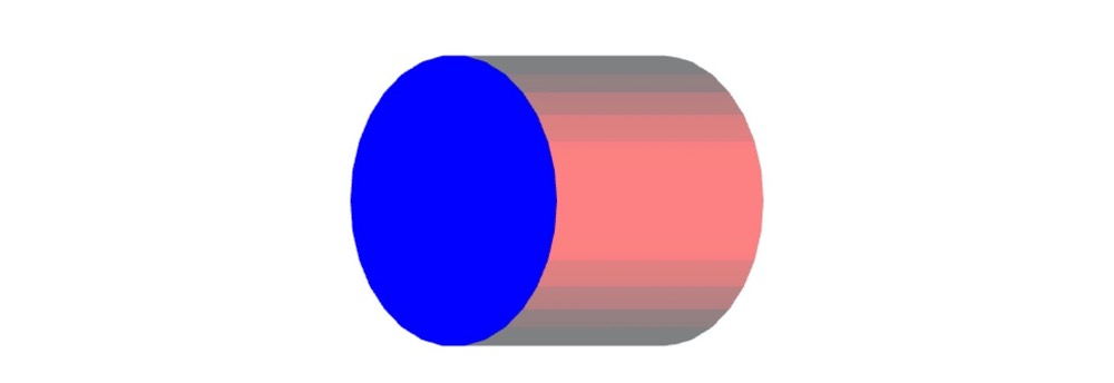
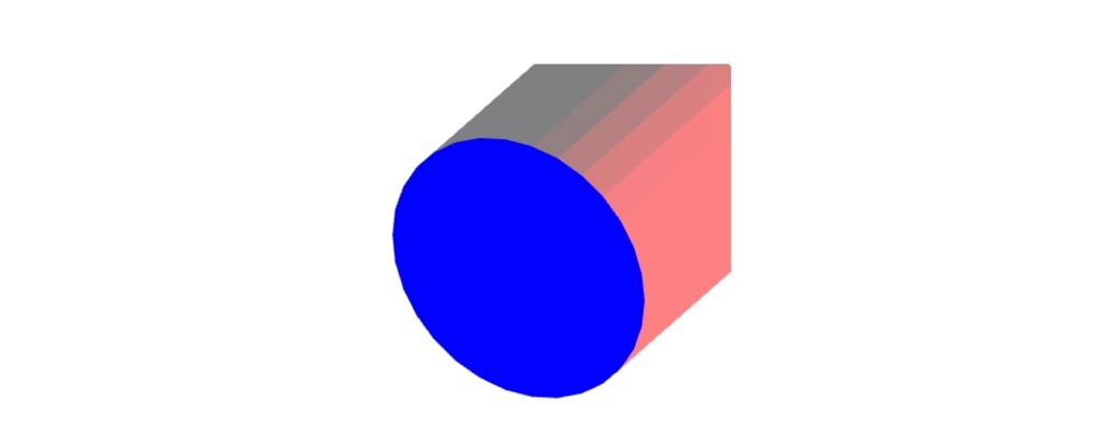
求出法向量,我们可以使用法向量来实现丰富的效果,比如点光源。下面,我们就在 shader 中实现点光源效果。
# 2. 法向量矩阵
因为我们在 shader 中,会使用模型矩阵对顶点进行变换,所以在片元着色器中,我们拿到的是变换后的顶点坐标,这时候,如果我们要应用法向量,需要对法向量也进行变换,我们可以通过一个矩阵来实现,这个矩阵叫做法向量矩阵(NormalMatrix)。它是模型矩阵的逆转置矩阵,不过它非常特殊,是一个 3X3 的矩阵(mat3),而像模型矩阵、投影矩阵等等矩阵都是 4X4 的。
得到了法向量和法向量矩阵,我们就可以使用法向量和法向量矩阵来实现点光源光照效果。
首先实现如下的顶点着色器:
attribute vec3 a_vertexPosition;
attribute vec4 color;
attribute vec3 normal;

varying vec4 vColor;
varying float vCos;
uniform mat4 projectionMatrix;
uniform mat4 modelMatrix;
uniform mat3 normalMatrix;

const vec3 lightPosition = vec3(1, 0, 0);

void main() {
  gl_PointSize = 1.0;
  vColor = color;
  vec4 pos =  modelMatrix * vec4(a_vertexPosition, 1.0);
  vec3 invLight = lightPosition - pos.xyz;
  vec3 norm = normalize(normalMatrix * normal);
  vCos = max(dot(normalize(invLight), norm), 0.0);
  gl_Position = projectionMatrix * pos;
}
2
3
4
5
6
7
8
9
10
11
12
13
14
15
16
17
18
19
20
21
在这段代码中,我们计算的是位于 (1,0,0) 坐标处的点光源与几何体法线的夹角余弦。那根据物体漫反射模型,光照强度等于光线与法向量夹角的余弦。
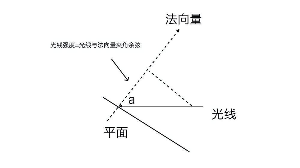
求出这个余弦值后,就能在片元着色器叠加光照了。最终效果看这里 (opens new window)。
#ifdef GL_ES
precision highp float;
#endif

uniform vec4 lightColor;
varying vec4 vColor;
varying float vCos;

void main() {
  gl_FragColor.rgb = vColor.rgb + vCos * lightColor.a * lightColor.rgb;
  gl_FragColor.a = vColor.a;
}
2
3
4
5
6
7
8
9
10
11
12
# 如何添加相机,用透视原理对物体进行投影
# 相机和视图矩阵
假设在 WebGL 的三维世界任意位置上有一个相机,它可以用一个三维坐标(Position)和一个三维向量方向(LookAt Target)来表示。
在初始情况下,相机的参考坐标和世界坐标是重合的。但是,当我们移动或者旋转相机的时候,相机的参考坐标和世界坐标就不重合了。
而我们最终要在 Canvas 画布上绘制出的是,以相机为观察者的图形,所以我们就需要用一个变换,将世界坐标转换为相机坐标。这个变换的矩阵就是视图矩阵(ViewMatrix)。
计算视图矩阵比较简单的一种方法是,我们先计算相机的模型矩阵,然后对矩阵使用 lookAt 函数,这样我们得到的矩阵就是视图矩阵的逆矩阵。然后,我们再对这个逆矩阵求一次逆,就可以得到视图矩阵了。
function updateCamera(eye, target = [0, 0, 0]) {
  const [x, y, z] = eye;
  const m = new Mat4( // 设置相机初始位置矩阵
    1, 0, 0, 0,
    0, 1, 0, 0,
    0, 0, 1, 0,
    x, y, z, 1,
  );
  const up = [0, 1, 0]; // up 是一个向量,表示朝上的方向,这里把它定义为 y 轴正向
  m.lookAt(eye, target, up).inverse(); // 将结果求逆,得到的就是视图矩阵
  renderer.uniforms.viewMatrix = m;
}
2
3
4
5
6
7
8
9
10
11
12
下面改写前面圆柱体的顶点着色器代码,加入视图矩阵。
attribute vec3 a_vertexPosition;
attribute vec4 color;
attribute vec3 normal;

varying vec4 vColor;
varying float vCos;
uniform mat4 projectionMatrix;
uniform mat4 modelMatrix;
uniform mat4 viewMatrix;
uniform mat3 normalMatrix;

const vec3 lightPosition = vec3(1, 0, 0);

void main() {
  gl_PointSize = 1.0;
  vColor = color;
  vec4 pos = viewMatrix * modelMatrix * vec4(a_vertexPosition, 1.0);
  vec4 lp = viewMatrix * vec4(lightPosition, 1.0);
  vec3 invLight = lp.xyz - pos.xyz;
  vec3 norm = normalize(normalMatrix * normal);
  vCos = max(dot(normalize(invLight), norm), 0.0);
  gl_Position = projectionMatrix * pos;
}
2
3
4
5
6
7
8
9
10
11
12
13
14
15
16
17
18
19
20
21
22
23
这样,如果我们改变相机的位置,比如:updateCamera([0.5, 0, 0.5]);,这样朝向 (0, 0, 0) 拍摄图像的最终效果如下。最终效果也可以看这里 (opens new window)。
# 剪裁空间和投影对 3D 图像的影响
WebGL 的默认坐标范围是从 -1 到 1 的。也就是说,只有当图像的 x、y、z 的值在 -1 到 1 区间内才会被显示在画布上,而在其他位置上的图像都会被剪裁掉。
比如,如果我们修改模型矩阵,让圆柱体沿 x、y 轴平移,向右上方各平移 0.5,那么圆柱中 x、y 值大于 1 的部分都会被剪裁掉,因为这些部分已经超过了 Canvas 边缘。
function update() {
  const modelMatrix = fromRotation(rotationX, rotationY, rotationZ);
  modelMatrix[12] = 0.5; // 给 x 轴增加 0.5 的平移
  modelMatrix[13] = 0.5; // 给 y 轴也增加 0.5 的平移
  renderer.uniforms.modelMatrix = modelMatrix;
  renderer.uniforms.normalMatrix = normalFromMat4([], modelMatrix);
  // ...
}
2
3
4
5
6
7
8
对于只有 x、y 的二维坐标系来说,这一点很好理解。但是,对于三维坐标系来说,不仅 x、y 轴会被剪裁,z 轴同样也会被剪裁。比如给 z 轴也增加 0.5 的平移,会看到最终绘制出来的图形非常奇怪。最终效果看这里 (opens new window)。
会显示这么奇怪的结果,就是因为 z 轴超过范围的部分也被剪裁掉了,导致投影出现了问题。
既然是投影出现了问题,我们先回想一下,我们都对 z 轴做过哪些投影操作。在绘制圆柱体的时候,我们只是用投影矩阵非常简单地反转了一下 z 轴,除此之外,没做过其他任何操作了。所以,为了让图形在剪裁空间中正确显示,我们不能只反转 z 轴,还需要将图像从三维空间中投影到剪裁坐标内。那么问题来了,图像是怎么被投影到剪裁坐标内的呢?
# 正投影和透视投影
一般来说,投影有两种方式,分别是正投影与透视投影。
正投影又叫做平行投影。正投影是将物体投影到一个长方体的空间(又称为视景体),并且无论相机与物体距离多远,投影的大小都不变。
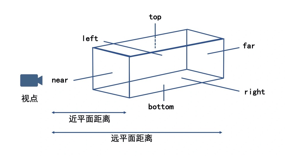
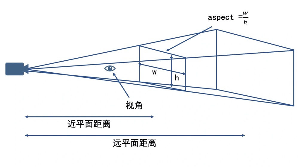
而透视投影则更接近我们的视觉感知。它投影的规律是,离相机近的物体大,离相机远的物体小。与正投影不同,正投影的视景体是一个长方体,而透视投影的视景体是一个棱台。
由于透视投影的效果更符合真实世界中我们看到的效果,所以一般来说,在绘制 3D 图形时,我们更偏向使用透视投影。
知道了不同投影方式的特点,我们就可以根据投影方式和给定的参数来计算投影矩阵了。只要记住下面 ortho 和 perspective 这两个投影函数就可以了。
// 计算正投影矩阵
// 参数是视景体 x、y、z 三个方向的坐标范围,它的返回值就是投影矩阵
function ortho(out, left, right, bottom, top, near, far) {
  let lr = 1 / (left - right);
  let bt = 1 / (bottom - top);
  let nf = 1 / (near - far);
  out[0] = -2 * lr;
  out[1] = 0;
  out[2] = 0;
  out[3] = 0;
  out[4] = 0;
  out[5] = -2 * bt;
  out[6] = 0;
  out[7] = 0;
  out[8] = 0;
  out[9] = 0;
  out[10] = 2 * nf;
  out[11] = 0;
  out[12] = (left + right) * lr;
  out[13] = (top + bottom) * bt;
  out[14] = (far + near) * nf;
  out[15] = 1;
  return out;
}

// 计算透视投影矩阵
// 参数是近景平面 near、远景平面 far、视角 fovy 和宽高比率 aspect,返回值也是投影矩阵
function perspective(out, fovy, aspect, near, far) {
  let f = 1.0 / Math.tan(fovy / 2);
  let nf = 1 / (near - far);
  out[0] = f / aspect;
  out[1] = 0;
  out[2] = 0;
  out[3] = 0;
  out[4] = 0;
  out[5] = f;
  out[6] = 0;
  out[7] = 0;
  out[8] = 0;
  out[9] = 0;
  out[10] = (far + near) * nf;
  out[11] = -1;
  out[12] = 0;
  out[13] = 0;
  out[14] = 2 * far * near * nf;
  out[15] = 0;
  return out;
}
2
3
4
5
6
7
8
9
10
11
12
13
14
15
16
17
18
19
20
21
22
23
24
25
26
27
28
29
30
31
32
33
34
35
36
37
38
39
40
41
42
43
44
45
46
47
48
# 对圆柱体进行正投影
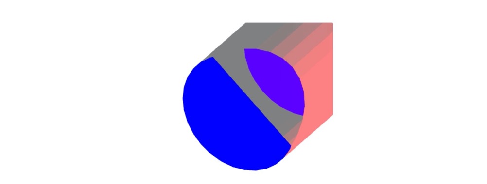
假设,在正投影的时候,我们让视景体三个方向的范围都是 (-2,2)。以刚才的相机位置为参照(任何一个位置观察都一样,不管物体在哪里,都是只有之前大小的一半。因为视景体范围增加了),我们绘制出来的圆柱体的大小只有之前的一半。这是因为我们通过投影变换将空间坐标范围增大了一倍。最终效果看这里 (opens new window)。
import {ortho} from '../common/lib/math/functions/Mat4Func.js';
function projection(left, right, bottom, top, near, far) {
  return ortho([], left, right, bottom, top, near, far);
}

const projectionMatrix = projection(-2, 2, -2, 2, -2, 2);
renderer.uniforms.projectionMatrix = projectionMatrix; // 投影矩阵

updateCamera([0.5, 0, 0.5]); // 设置相机位置
2
3
4
5
6
7
8
9
# 对圆柱体进行透视投影
最终效果看这里 (opens new window)。
import {perspective} from '../common/lib/math/functions/Mat4Func.js';

function projection(near = 0.1, far = 100, fov = 45, aspect = 1) {
  return perspective([], fov * Math.PI / 180, aspect, near, far);
}

const projectionMatrix = projection();
renderer.uniforms.projectionMatrix = projectionMatrix;

updateCamera([2, 2, 3]); // 设置相机位置
2
3
4
5
6
7
8
9
10
# 3D 绘图标准模型
3D 绘图的标准模型一共有四个矩阵,它们分别是:投影矩阵、视图矩阵(ViewMatrix)、模型矩阵(ModelMatrix)、法向量矩阵(NormalMatrix)。
其中,前三个矩阵用来计算最终显示的几何体的顶点位置,第四个矩阵用来实现光照等效果。
比较成熟的图形库,如 ThreeJS (opens new window)、BabylonJS (opens new window),基本上都是采用这个标准模型来进行 3D 绘图的。所以理解这个模型,也有助于增强我们对图形库的认识,帮助我们更好地去使用这些流行的图形库。
# 轻量级的图形库:OGL
之前我们使用 gl-renderer (opens new window) 库来简化 2D 绘图过程,而 3D 绘图是一个比 2D 绘图更加复杂的过程,即使是 gl-renderer 库也有点力不从心,我们需要更加强大的绘图库,来简化我们的绘制,以便于我们能够把精力专注于理解图形学本身的核心内容。
这里可以使用 OGL (opens new window),它拥有我们可视化绘图需要的所有基本功能,而且,相比于 ThreeJS 等流行图形库,它的 AP 相对更底层、更简单一些。
# 使用 OGL 绘制基本的几何体
OGL 绘制几何体分为以下 7 个步骤:
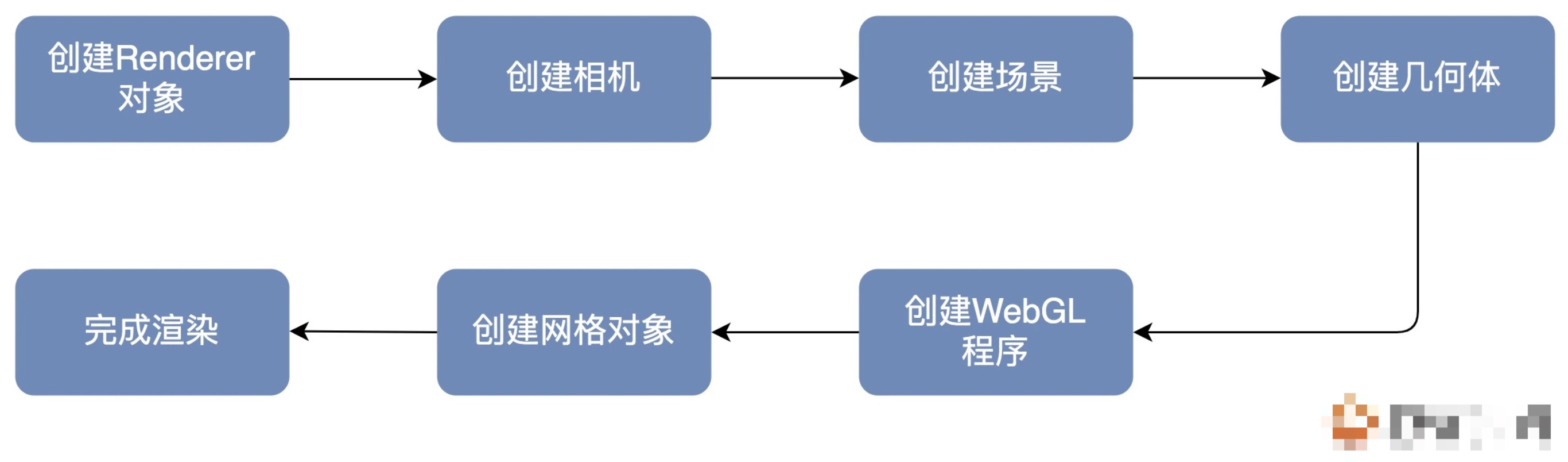
首先,是创建 Renderer 对象。我们可以创建一个画布宽高为 512 的 Renderer 对象。
const canvas = document.querySelector('canvas');
const renderer = new Renderer({
  canvas,
  width: 512,
  height: 512,
});
2
3
4
5
6
然后,我们在 OGL 中,通过 new Camera 来创建相机,默认创建出的是透视投影相机。这里我们把视角设置为 35 度,位置设置为 (0,1,7),朝向为 (0,0,0)。
const gl = renderer.gl;
gl.clearColor(1, 1, 1, 1);
const camera = new Camera(gl, {fov: 35});
camera.position.set(0, 1, 7);
camera.lookAt([0, 0, 0]);
2
3
4
5
接着,我们创建场景。OGL 使用树形渲染的方式,所以在用 OGL 创建场景时,我们要使用 Transform 元素。Transform 类型是基本元素,它可以添加子元素和设置几何变换,如果父元素设置了变换,这些变换也会被应用到子元素。
const scene = new Transform();
然后,我们创建几何体对象。OGL 内置了许多常用的几何体对象,包括球体 Sphere、立方体 Box、柱 / 锥体 Cylinder 以及环面 Torus 等等。使用这些对象,我们可以快速创建这些几何体的顶点信息。这里创建了 4 个几何体对象,分别是球体、立方体、椎体和环面。
const sphereGeometry = new Sphere(gl);
const cubeGeometry = new Box(gl);
const cylinderGeometry = new Cylinder(gl);
const torusGeometry = new Torus(gl);
2
3
4
再然后,我们创建 WebGL 程序。并且,我们在着色器中给这些几何体设置了浅蓝色和简单的光照效果。
const vertex = /* glsl */ `
  precision highp float;

  attribute vec3 position;
  attribute vec3 normal;
  uniform mat4 modelViewMatrix;
  uniform mat4 projectionMatrix;
  uniform mat3 normalMatrix;
  varying vec3 vNormal;
  void main() {
    vNormal = normalize(normalMatrix * normal);
    gl_Position = projectionMatrix * modelViewMatrix * vec4(position, 1.0);
  }
`;

const fragment = /* glsl */ `
  precision highp float;

  varying vec3 vNormal;
  void main() {
    vec3 normal = normalize(vNormal);
    float lighting = dot(normal, normalize(vec3(-0.3, 0.8, 0.6)));
    gl_FragColor.rgb = vec3(0.2, 0.8, 1.0) + lighting * 0.1;
    gl_FragColor.a = 1.0;
  }
`;

const program = new Program(gl, {
  vertex,
  fragment,
});
2
3
4
5
6
7
8
9
10
11
12
13
14
15
16
17
18
19
20
21
22
23
24
25
26
27
28
29
30
31
有了 WebGL 程序之后,我们就可以使用它和几何体对象来构建真正的网格(Mesh)元素,最终再把这些元素渲染到画布上。我们创建了 4 个网格对象,它们的形状分别是环面、球体、立方体和圆柱,给它们设置了不同的位置,然后将它们添加到场景 scene 中去。
const torus = new Mesh(gl, {geometry: torusGeometry, program});
torus.position.set(0, 1.3, 0);
torus.setParent(scene);

const sphere = new Mesh(gl, {geometry: sphereGeometry, program});
sphere.position.set(1.3, 0, 0);
sphere.setParent(scene);

const cube = new Mesh(gl, {geometry: cubeGeometry, program});
cube.position.set(0, -1.3, 0);
cube.setParent(scene);

const cylinder = new Mesh(gl, {geometry: cylinderGeometry, program});
cylinder.position.set(-1.3, 0, 0);
cylinder.setParent(scene);
2
3
4
5
6
7
8
9
10
11
12
13
14
15
最后,我们将它们用相机 camera 对象的设定渲染出来,并分别设置绕 y 轴旋转的动画,最终效果看这里 (opens new window)。
requestAnimationFrame(update);
function update() {
  requestAnimationFrame(update);

  torus.rotation.y -= 0.02;
  sphere.rotation.y -= 0.03;
  cube.rotation.y -= 0.04;
  cylinder.rotation.y -= 0.02;

  renderer.render({scene, camera});
}
2
3
4
5
6
7
8
9
10
11

# 如何用仿射变换来移动和旋转 3D 物体
在前面,我们用仿射变换来移动和旋转二维图形。在三维世界中,想要移动和旋转物体,我们也需要使用仿射变换。
# 三维仿射变换
三维仿射变换和二维仿射变换类似,也包括平移、旋转与缩放等等,而且具体的变换公式也相似。
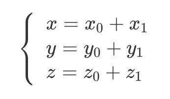
# 平移变换
对于平移变换来说,如果向量
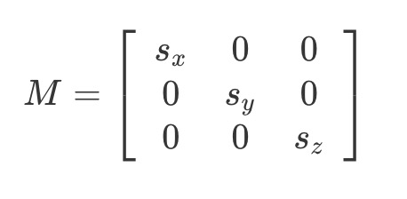
# 缩放变换
对于缩放变换来说,我们直接让三维向量乘上标量,就相当于乘上要缩放的倍数就可以了。最后我们得到的三维缩放变换矩阵如下:
# 齐次矩阵表示三维仿射变换
此外,我们也可以使用齐次矩阵来表示三维仿射变换,通过引入一个新的维度,就可以把仿射变换转换为齐次矩阵的线性变换了。

这个齐次矩阵,是一个 4X4 的矩阵,其实它就是我们在之前提到的模型矩阵(ModelMatrix)。
总之,对于三维的仿射变换来说,平移和缩放都只是增加一个 z 分量,这和二维放射变换没有什么不同。
但对于物体的旋转变换,三维就要比二维稍微复杂一些了。因为二维旋转只有一个参考轴,就是 z 轴,所以二维图形旋转都是围绕着 z 轴的。但是,三维物体的旋转却可以围绕 x、y、z,这三个轴其中任意一个轴来旋转。
# 旋转变换
# 欧拉角
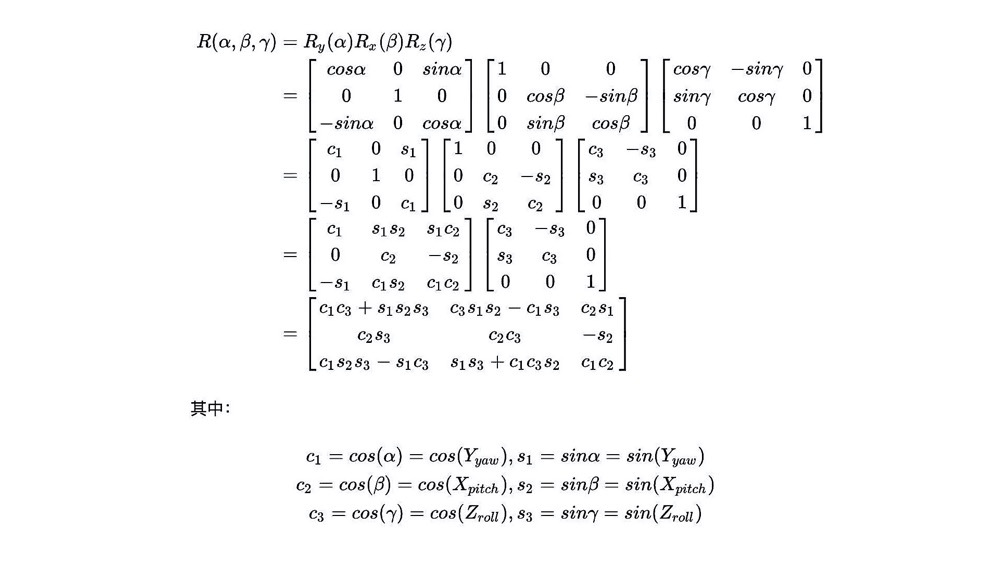
三维物体的旋转变换矩阵如下:
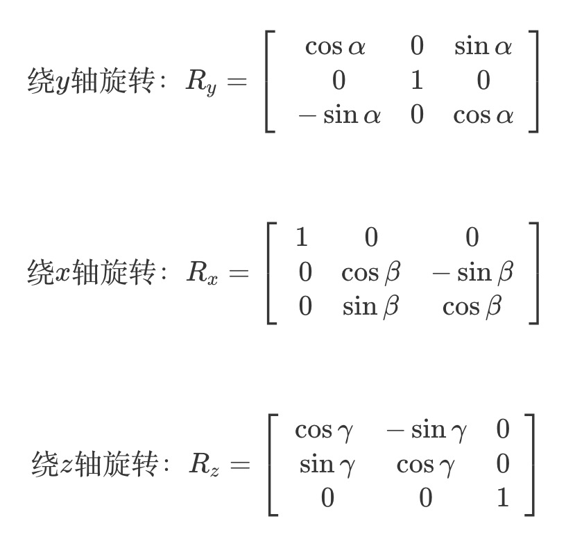
可以看到,我们使用了三个旋转矩阵
# 什么是欧拉角
欧拉角是描述三维物体在空间中取向的标准数学模型,也是航空航天普遍采用的标准。对于在三维空间里的一个参考系,任何坐标系的取向,都可以用三个欧拉角来表示。
比如,下图中这个飞机的飞行姿态,可以由绕 x 轴的旋转角度(翻滚机身)、绕 y 轴的旋转角度(俯仰),以及绕 z 轴的旋转角度(偏航)来表示。
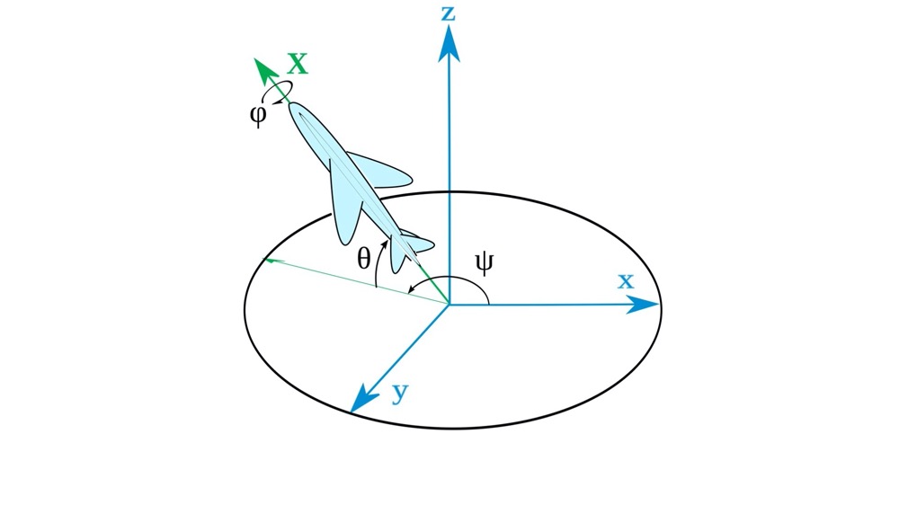
也就是说,这个飞机的姿态可以由这三个欧拉角来确定。具体的表示公式就是
这里,我们是按照
# 欧拉角的顺规
欧拉角有很多种不同的顺规表示方式,一共可以分两种。不同的欧拉角顺规虽然表示方法不同,但它们本质上还是欧拉角,都可以表示三维几何空间中的任意取向。所以,我们在绘制三维图形的时候,使用任何一种表示法都可以。
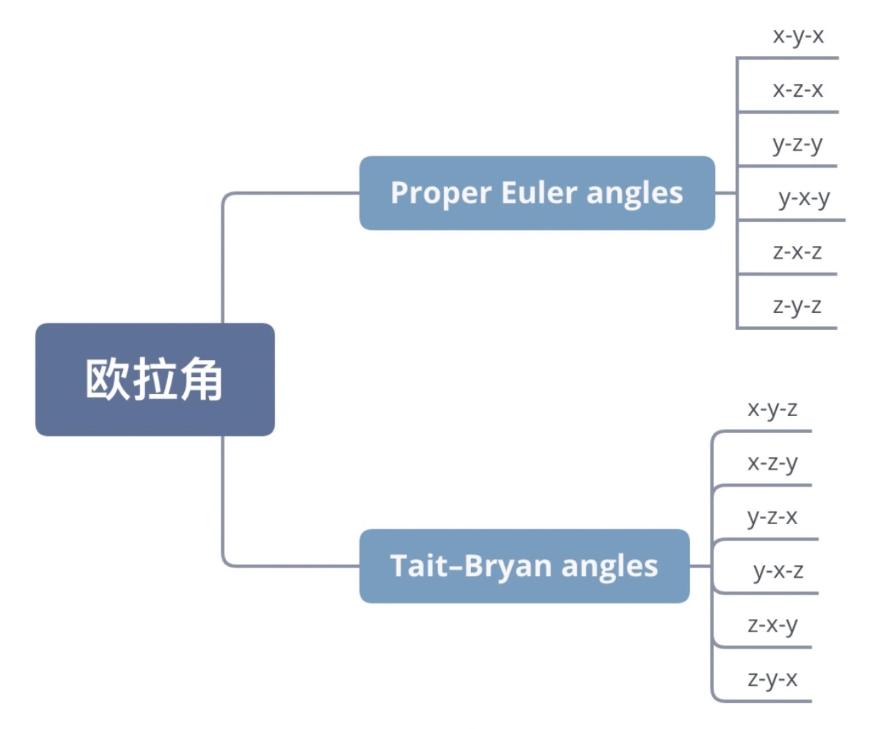
采用 y−x−z 顺规的欧拉角之后,我们就能得到如下的旋转矩阵结果:
# 使用欧拉角来旋转几何体
下面使用 OGL (opens new window) 来演示使用欧拉角来旋转几何体的具体过程。
OGL 的几何网格(Mesh)对象直接支持欧拉角,我们直接用对象的 rotation 属性就可以设置欧拉角,rotation 属性是一个三维向量,它的 x、y、z 坐标就对应围绕 x、y、z 旋转的欧拉角。而且 OGL 框架默认的欧拉角顺规是 y−x−z。
在 OGL 中,我们可以加载 JSON 文件,来载入预先设计好的飞机几何模型 (opens new window)。
下面是一个封装好的用来记载几何模型的函数。这个函数会载入 JSON 文件的内容,然后根据其中的数据创建 Geometry 对象,并返回这个对象。
async function loadModel(src) {
  const data = await (await fetch(src)).json();

  const geometry = new Geometry(gl, {
    position: {size: 3, data: new Float32Array(data.position)},
    uv: {size: 2, data: new Float32Array(data.uv)},
    normal: {size: 3, data: new Float32Array(data.normal)},
  });

  return geometry;
}

const geometry = await loadModel('../assets/airplane.json'); // 加载飞机几何模型
2
3
4
5
6
7
8
9
10
11
12
13
飞机几何模型数据如下,其中 position、normal、uv 是顶点数据,分别是顶点坐标、法向量和纹理坐标。这样的数据一般是由设计工具直接生成的,不需要我们来计算。
{
  "position": [0.752, 1.061, 0.0, 0.767...],
  "normal": [0.975, 0.224, 0.0, 0.975...],
  "uv": [0.745, 0.782, 0.705, 0.769...]
}
2
3
4
5
接下来,我们加载飞机的纹理图片 (opens new window),同样要先封装一个加载图片纹理的函数。在函数里,我们用 img 元素加载图片,然后将图片赋给对应的纹理对象。
function loadTexture(src) {
  const texture = new Texture(gl);
  return new Promise((resolve) => {
    const img = new Image();
    img.onload = () => {
      texture.image = img;
      resolve(texture);
    };
    img.src = src;
  });
}


const texture = await loadTexture('../assets/airplane.jpg'); // 加载飞机的纹理图片
2
3
4
5
6
7
8
9
10
11
12
13
14
然后,我们在片元着色器中,直接读取纹理图片中的颜色信息。
precision highp float;

uniform sampler2D tMap;
varying vec2 vUv;

void main() {
  gl_FragColor = texture2D(tMap, vUv);
}
2
3
4
5
6
7
8
最后,我们就能将元素渲染出来了。渲染指令如下:
const program = new Program(gl, {
  vertex,
  fragment,
  uniforms: {
    tMap: {value: texture},
  },
});
const mesh = new Mesh(gl, {geometry, program});
mesh.setParent(scene);
renderer.render({scene, camera});
2
3
4
5
6
7
8
9
10
最终,我们就能得到可以随意调整欧拉角的飞机模型了,效果看这里 (opens new window)。
# 万向节锁
使用欧拉角来操作几何体的方向,虽然很简单,但是有一个小缺陷,这个缺陷叫做万向节锁 (Gimbal Lock)。
在上面的飞机例子中,当我们分别改变飞机的 alpha、beta、theta 值时,飞机会做出对应的姿态调整,包括偏航(改变 alpha)、翻滚(改变 beta)和俯仰(改变 theta)。
但是如果我们将 beta 固定在正负 90 度,改变 alpha 和 beta,我们会发现一个奇特的现象:
此时,不管改变 alpha 还是改变 theta,飞机都绕着 y 轴旋转,始终处于一个平面上。也就是说,本来飞机姿态有 x、y、z 三个自由度,现在 y 轴被固定了,只剩下两个自由度了,这就是万向节锁。
万向节锁,并不是真的 “锁” 住。而是在特定的欧拉角情况下,姿态调整的自由度丢失了。而且,只要是欧拉角,不管我们使用哪一种顺规,万向节锁都会存在。
# 四元数
四元数是一种高阶复数,一个四元数可以表示为:
我们可以用单位四元数来描述 3D 旋转。所谓单位四元数,就是其中的参数满足
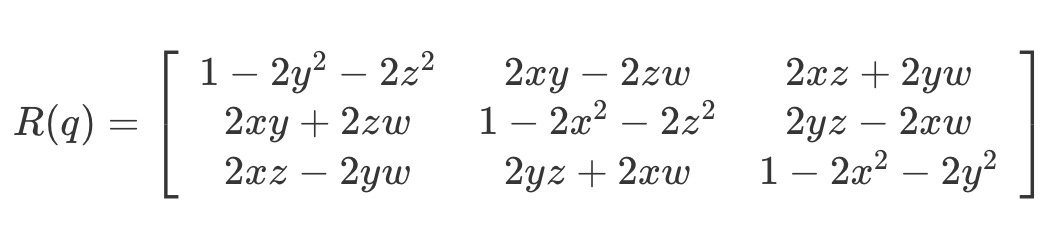
这个旋转矩阵的数学推导过程 (opens new window)比较复杂,我们只要记住这个公式就行了。
# 四元数vs欧拉角vs旋转矩阵
与欧拉角相比,四元数没有万向节死锁的问题。而且与旋转矩阵相比,四元数只需要四个分量就可以定义,模型上更加简洁。但是,四元数相对来说没有旋转矩阵和欧拉角那么直观。
# 四元数与轴角
四元数有一个常见的用途是用来处理轴角。
所谓轴角,就是在三维空间中,给定一个由单位向量表示的轴,以及一个旋转角度 ⍺,以此来表示几何体绕该轴旋转 ⍺ 角。
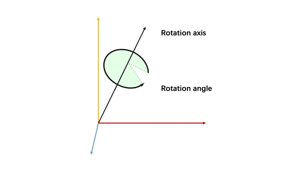
绕单位向量 u 旋转 ⍺ 角,对应的四元数可以表示为:
下面是一个四元数处理轴角的例子。
还是以前面飞机为例,不过,这次我们将欧拉角换成轴角,实现一个 updateAxis 和 updateQuaternion 函数,分别更新轴和四元数。
// 更新轴
function updateAxis() {
  const {x, y, z} = palette;
  const v = new Vec3(x, y, z).normalize().scale(10);
  points[1].copy(v);
  axis.updateGeometry();
  renderer.render({scene, camera});
}

// 更新四元数
function updateQuaternion(val) {
  const theta = 0.5 * val / 180 * Math.PI;
  const c = Math.cos(theta);
  const s = Math.sin(theta);
  const p = new Vec3().copy(points[1]).normalize();
  const q = new Quat(p.x * s, p.y * s, p.z * s, c);
  mesh.quaternion = q;
  renderer.render({scene, camera});
}
2
3
4
5
6
7
8
9
10
11
12
13
14
15
16
17
18
19
然后,我们定义轴, 再把它显示出来。在 OGL 里面,我们可以通过 Polyline 对象来绘制轴。
const points = [
  new Vec3(0, 0, 0),
  new Vec3(0, 10, 0),
];

const axis = new Polyline(gl, {
  points,
  uniforms: {
    uColor: {value: new Color('#f00')},
    uThickness: {value: 3},
  },
});
axis.mesh.setParent(scene);
2
3
4
5
6
7
8
9
10
11
12
13
这样,我们就实现了用四元数让飞机沿着某个轴旋转的效果了,最终效果看这里 (opens new window)。这其中最重要的一步,是要你理解怎么根据旋转轴和轴角来计算对应的四元数,也就是 updateQuaternion 函数里面做的事情。然后我们将这个更新后的四元数赋给飞机的 mesh 对象,就可以更新飞机的位置,实现飞机绕轴的旋转。
# 更多学习资料
# 如何模拟光照让 3D 场景更逼真
物体的光照效果是由光源、介质(物体的材质)和反射类型决定的,而反射类型又由物体的材质特点决定。
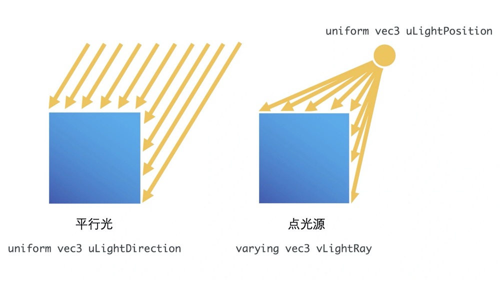
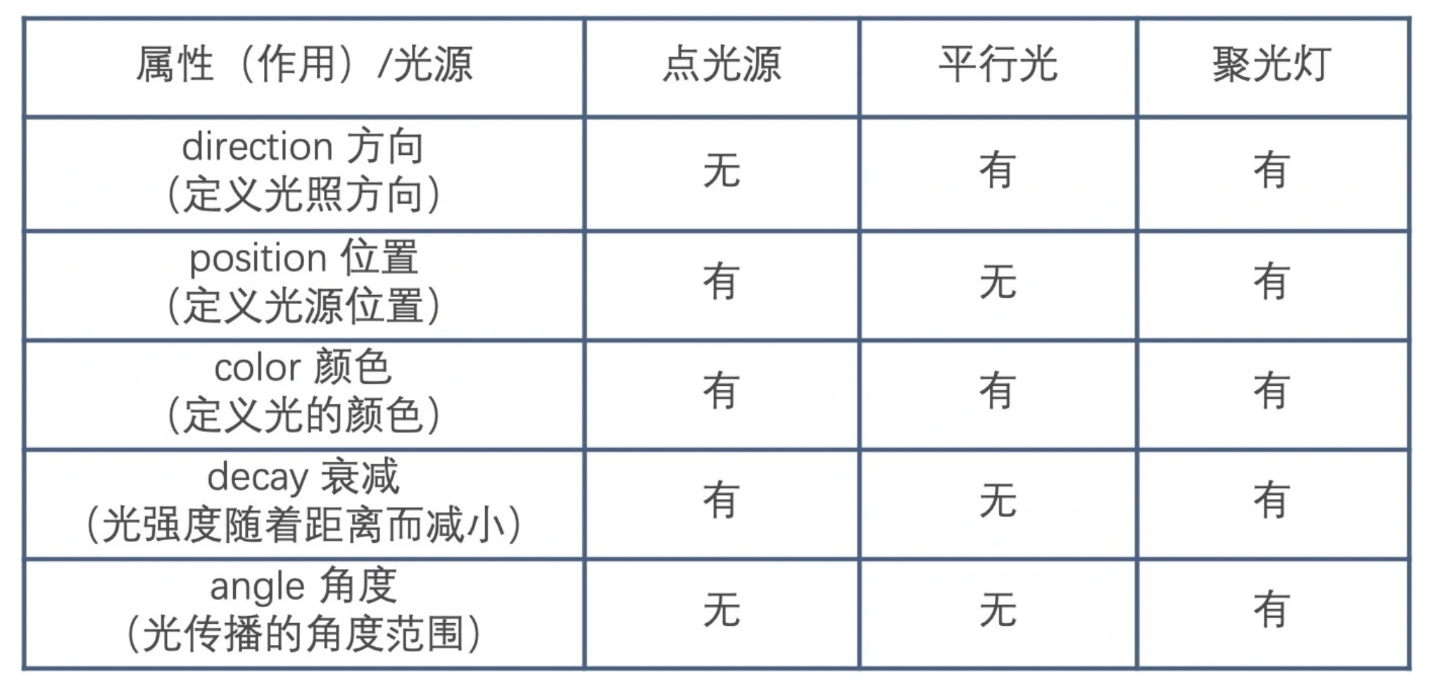
在 3D 光照模型中,根据不同的光源特点,我们可以将光源分为 4 种不同的类型,分别是环境光(Ambient Light)、平行光(Directional Light)、点光源(Positional Light)和聚光灯(Spot Light)。而物体的反射类型,则分为漫反射和镜面反射两种。
# 环境光
环境光就是指物体所在的三维空间中天然的光,它充满整个空间,在每一处的光照强度都一样。
环境光没有方向,所以,物体表面反射环境光的效果,只和环境光本身以及材质的反射率有关。
环境光有以下两个特点:
因为它在空间中均匀分布,所以在任何位置上环境光的颜色都相同。
它与物体的材质有关。如果物体的 RGB 通道反射率不同的话,那么它在相同的环境光下就会呈现出不同的颜色。因此,如果环境光是白光(#FFF),那么物体呈现的颜色就是材质反射率表现出的颜色,也就是物体的固有颜色。
# 如何添加环境光效果
物体在环境光中呈现的颜色,我们可以利用下面的公式来求。其中,环境光的颜色为 L,材质对光的反射率为 R。
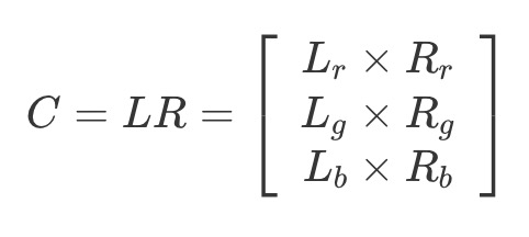
创建一个着色器,用这个着色器创建 WebGL 着色器程序,传入环境光 ambientLight 和材质反射率 materialReflection,就可以渲染出各种颜色的几何体了。最终效果看这里 (opens new window)。
precision highp float;

uniform vec3 ambientLight;
uniform vec3 materialReflection;

void main() {
  gl_FragColor.rgb = ambientLight * materialReflection;
  gl_FragColor.a = 1.0;
}
2
3
4
5
6
7
8
9
# 颜色属性和光照模型的对比
那通过这样渲染出来的几何体颜色,与我们之前通过设置颜色属性得到的颜色有什么区别呢?
在前面,我们绘制的几何体只有颜色属性,但是在光照模型里,我们把颜色变为了环境光和反射率两个属性。这样的模型更加接近于真实世界,也让物体的颜色有了更灵活的控制手段。比如,我们修改环境光,就可以改变整个画布上所有受光照模型影响的几何体的颜色,而如果只是像之前那样给物体分别设置颜色,我们就只能一一修改这些物体各自的颜色了。
# 平行光
与环境光不同,平行光是朝着某个方向照射的光,它能够照亮几何体的一部分表面。
平行光除了颜色这个属性之外,还有方向,它属于有向光。
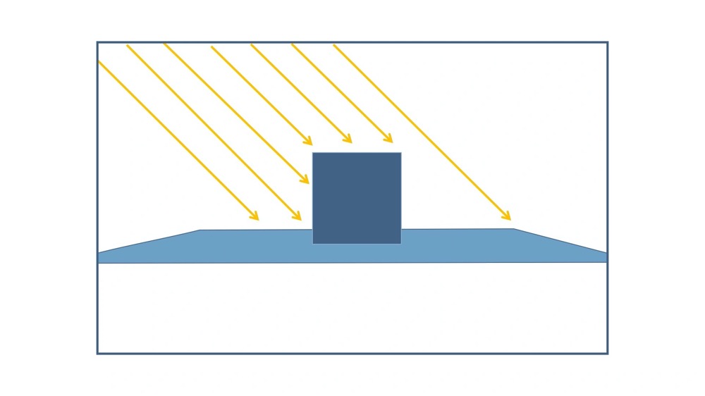
有向光在与物体发生作用的时候,根据物体的材质特性,会产生两种反射,一种叫做漫反射(Diffuse reflection),另一种叫做镜面反射(Specular reflection),而一个物体最终的光照效果,是漫反射、镜面反射以及环境光叠加在一起的效果。
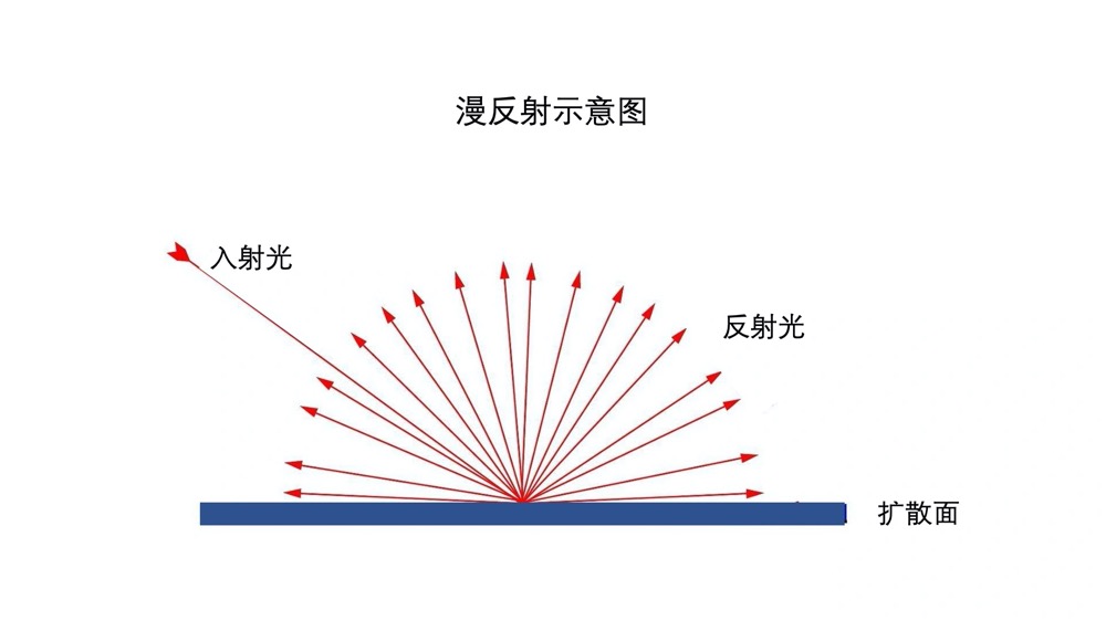
有向光的漫反射在各个方向上的反射光均匀分布,反射强度与光的射入方向与法线的夹角的余弦成正比。
# 如何添加平行光效果
下面演示下如何添加一道白色的平行光。
首先,我们在顶点着色器中添加一道平行光。具体来说就是传入一个 directionalLight 向量。为什么是顶点着色器呢?因为,我们在顶点着色器中计算光线的方向,需要运算的次数少,会比在片元着色器中计算的性能要好很多。
precision highp float;

attribute vec3 position;
attribute vec3 normal;
uniform mat4 modelViewMatrix;
uniform mat4 projectionMatrix;
uniform mat4 viewMatrix;
uniform mat3 normalMatrix;
uniform vec3 directionalLight;

varying vec3 vNormal;
varying vec3 vDir;

void main() {
  // 计算光线方向
  vec4 invDirectional = viewMatrix * vec4(directionalLight, 0.0);
  vDir = -invDirectional.xyz;

  // 计算法向量
  vNormal = normalize(normalMatrix * normal);
  gl_Position = projectionMatrix * modelViewMatrix * vec4(position, 1.0);
}
2
3
4
5
6
7
8
9
10
11
12
13
14
15
16
17
18
19
20
21
22
然后,在片元着色器里,我们计算光线方向与法向量夹角的余弦,计算出漫反射光。在平行光下,物体最终呈现的颜色是环境光加上漫反射光与材质反射率的乘积。
precision highp float;

uniform vec3 ambientLight;
uniform vec3 materialReflection;
uniform vec3 directionalLightColor;

varying vec3 vNormal;
varying vec3 vDir;

void main() {
  // 求光线与法线夹角的余弦
  float cos = max(dot(normalize(vDir), vNormal), 0.0);

  // 计算漫反射
  vec3 diffuse = cos * directionalLightColor;

  // 合成颜色
  gl_FragColor.rgb = (ambientLight + diffuse) * materialReflection;
  gl_FragColor.a = 1.0;
}
2
3
4
5
6
7
8
9
10
11
12
13
14
15
16
17
18
19
20
接着,我们在 JavaScript 代码里,给 WebGL 程序添加一个水平向右的白色平行光。
const ambientLight = {value: [0.5, 0.5, 0.5]};

const directional = {
  directionalLight: {value: [1, 0, 0]},
  directionalLightColor: {value: [1, 1, 1]},
};

const program1 = new Program(gl, {
  vertex,
  fragment,
  uniforms: {
    ambientLight,
    materialReflection: {value: [0, 0, 1]},
    ...directional,
  },
});
// ...
2
3
4
5
6
7
8
9
10
11
12
13
14
15
16
17
最终显示的效果如下,也可以看这里 (opens new window)。当旋转相机位置的时候,我们看到物体因为光照,不同方向表面的明暗度不一样。
# 点光源
点光源就是指空间中某一点发出的光,与方向光不同的是,点光源不仅有方向属性,还有位置属性。
因此计算点光源的光照,我们要先根据光源位置和物体表面相对位置来确定方向,然后再和平行光一样,计算光的方向和物体表面法向的夹角。计算过程要比平行光稍微复杂一些。
# 如何添加点光源效果
对于平行光来说,只要法向量相同,方向就相同,所以我们可以直接在顶点着色器中计算方向。
但点光源因为其方向与物体表面的相对位置有关,所以我们不能在顶点着色器中计算,需要在片元着色器中计算。
因此,计算点光源光照效果的第一步,就是要在顶点着色器中,将物体变换后的坐标传给片元着色器。
precision highp float;

attribute vec3 position;
attribute vec3 normal;
uniform mat4 modelViewMatrix;
uniform mat4 projectionMatrix;
uniform mat3 normalMatrix;

varying vec3 vNormal;
varying vec3 vPos;

void main() {
  vPos = modelViewMatrix * vec4(position, 1.0);
  vNormal = normalize(normalMatrix * normal);
  gl_Position = projectionMatrix * vPos;
}
2
3
4
5
6
7
8
9
10
11
12
13
14
15
16
接下来,片元着色器中的计算过程就和平行光类似了。 我们要计算光线方向与法向量夹角的余弦,用 (viewMatrix * vec4(pointLightPosition, 1.0)).xyz - vPos 得出点光源与当前位置的向量,然后用这个向量和法向量计算余弦值,这样就得到了我们需要的漫反射余弦值。
precision highp float;

uniform vec3 ambientLight;
uniform vec3 materialReflection;
uniform vec3 pointLightColor;
uniform vec3 pointLightPosition;
uniform mat4 viewMatrix;

varying vec3 vNormal;
varying vec3 vPos;

void main() {
  // 光线到点坐标的方向
  vec3 dir = (viewMatrix * vec4(pointLightPosition, 1.0)).xyz - vPos;

  // 与法线夹角余弦
  float cos = max(dot(normalize(dir), vNormal), 0.0);

  // 计算漫反射
  vec3 diffuse = cos * pointLightColor;

  // 合成颜色
  gl_FragColor.rgb = (ambientLight + diffuse) * materialReflection;
  gl_FragColor.a = 1.0;
}
2
3
4
5
6
7
8
9
10
11
12
13
14
15
16
17
18
19
20
21
22
23
24
25
假设我们将点光源设置在 (3,3,0) 位置,颜色为白光,得到的效果如下。
# 点光源的衰减
不过,前面的计算过程都是理想状态下的。而真实世界中,点光源的光照强度会随着空间的距离增加而衰减。所以,为了实现更逼真的效果,我们必须要把光线衰减程度也考虑进去。
光线的衰减程度,我们一般用衰减系数表示。衰减系数等于一个常量
一般来说,衰减函数可以用一个二次多项式 P 来描述,它的计算公式为:
其中 A、B、C 为常量,它们的取值会根据实际的需要随时变化,z 是当前位置到点光源的距离。
接下来,我们需要在片元着色器中增加衰减系数。在计算的时候,我们必须要提供光线到点坐标的距离。
precision highp float;

uniform vec3 ambientLight;
uniform vec3 materialReflection;
uniform vec3 pointLightColor;
uniform vec3 pointLightPosition;
uniform mat4 viewMatrix;
uniform vec3 pointLightDecayFactor;

varying vec3 vNormal;
varying vec3 vPos;

void main() {
  // 光线到点坐标的方向
  vec3 dir = (viewMatrix * vec4(pointLightPosition, 1.0)).xyz - vPos;

  // 光线到点坐标的距离,用来计算衰减
  float dis = length(dir);

  // 与法线夹角余弦
  float cos = max(dot(normalize(dir), vNormal), 0.0);

  // 计算衰减
  float decay = min(1.0, 1.0 /
    (pointLightDecayFactor.x * pow(dis, 2.0) + pointLightDecayFactor.y * dis + pointLightDecayFactor.z));

  // 计算漫反射
  vec3 diffuse = decay * cos * pointLightColor;

  // 合成颜色
  gl_FragColor.rgb = (ambientLight + diffuse) * materialReflection;
  gl_FragColor.a = 1.0;
}
2
3
4
5
6
7
8
9
10
11
12
13
14
15
16
17
18
19
20
21
22
23
24
25
26
27
28
29
30
31
32
33
假设,我们将衰减系数设置为 (0.05, 0, 1),就能得到如下效果,也可以看这里 (opens new window)。把它和前一张图对比,会发现,我们看到较远的几何体几乎没有光照了。这就是因为光线强度随着距离衰减了,也就更接近真实世界的效果。
# 聚光灯
与点光源相比,聚光灯增加了方向以及角度范围,只有在这个范围内,光线才能照到。
那该如何判断坐标是否在角度范围内呢?
我们可以根据法向量与光线方向夹角的余弦值来判断坐标是否在夹角内,之前用向量乘法判断点是否处于扫描范围内,这里就是具体应用。
最终片元着色器中的代码如下:
precision highp float;

uniform mat4 viewMatrix;
uniform vec3 ambientLight;
uniform vec3 materialReflection;
uniform vec3 spotLightColor; // 聚光灯颜色
uniform vec3 spotLightPosition; // 聚光灯位置
uniform vec3 spotLightDecayFactor; // 聚光灯衰减系数
uniform vec3 spotLightDirection; // 聚光灯方向
uniform float spotLightAngle; // 聚光灯角度

varying vec3 vNormal;
varying vec3 vPos;

void main() {
  // 光线到点坐标的方向
  vec3 invLight = (viewMatrix * vec4(spotLightPosition, 1.0)).xyz - vPos;
  vec3 invNormal = normalize(invLight);

  // 光线到点坐标的距离,用来计算衰减
  float dis = length(invLight);
  // 聚光灯的朝向
  vec3 dir = (viewMatrix * vec4(spotLightDirection, 0.0)).xyz;

  // 通过余弦值判断夹角范围
  float ang = cos(spotLightAngle);
  float r = step(ang, dot(invNormal, normalize(-dir)));

  // 与法线夹角余弦
  float cos = max(dot(invNormal, vNormal), 0.0);
  // 计算衰减
  float decay = min(1.0, 1.0 /
    (spotLightDecayFactor.x * pow(dis, 2.0) + spotLightDecayFactor.y * dis + spotLightDecayFactor.z));

  // 计算漫反射
  vec3 diffuse = r * decay * cos * spotLightColor;

  // 合成颜色
  gl_FragColor.rgb = (ambientLight + diffuse) * materialReflection;
  gl_FragColor.a = 1.0;
}
2
3
4
5
6
7
8
9
10
11
12
13
14
15
16
17
18
19
20
21
22
23
24
25
26
27
28
29
30
31
32
33
34
35
36
37
38
39
40
41
在计算光线和法线夹角的余弦值时,我们是用与点光源一样的方式。此外,我们还增加了一个步骤,就是以聚光灯方向和角度,计算点坐标是否在光照角度内。如果在,那么 r 的值是 1,否则 r 的值是 0。
假设我们是这样设置的,那么最终的光照效果就只会出现在光照的角度内。
const directional = {
  spotLightPosition: {value: [3, 3, 0]},
  spotLightColor: {value: [1, 1, 1]},
  spotLightDecayFactor: {value: [0.05, 0, 1]},
  spotLightDirection: {value: [-1, -1, 0]},
  spotLightAngle: {value: Math.PI / 12},
};
2
3
4
5
6
7
我们最终渲染出来的结果如下,也可以看这里 (opens new window)。
# 镜面反射
前面介绍了四种光照的漫反射模型。实际上,因为物体的表面材质不同,反射光不仅有漫反射,还有镜面反射。
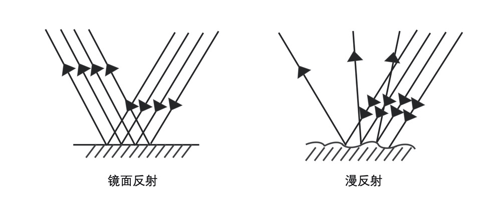
如果若干平行光照射在表面光滑的物体上,反射出来的光依然平行,这种反射就是镜面反射。镜面反射的性质是,入射光与法线的夹角等于反射光与法线的夹角。
越光滑的材质,它的镜面反射效果也就越强。最直接的表现就是物体表面会有闪耀的光斑,也叫镜面高光。
但并不是所有光都能产生镜面反射,环境光因为没有方向,所以不参与镜面反射。剩下的平行光、点光源、聚光灯这三种光源,都是能够产生镜面反射的有向光。
# 如何实现有向光的镜面反射
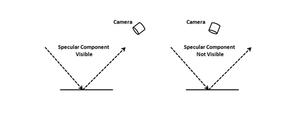
首先,镜面反射需要同时考虑光的入射方向以及相机也就是观察者所在的方向。
实现镜面反射效果一般来说需要 4 个步骤:
第一步,求出反射光线的方向向量。这里我们以点光源为例,要求出反射光的方向,我们可以直接使用 GLSL 的内置函数 reflect,这个函数能够返回一个向量相对于某个法向量的反射向量,正好就是我们要的镜面反射结果。
// 求光源与点坐标的方向向量
vec3 dir = (viewMatrix * vec4(pointLightPosition, 1.0)).xyz - vPos;

// 归一化
dir = normalize(dir);

// 求反射向量
vec3 reflectionLight = reflect(-dir, vNormal);
2
3
4
5
6
7
8
第二步,我们要根据相机位置计算视线与反射光线夹角的余弦,用到原理是向量的点乘。
vec3 eyeDirection = vCameraPos - vPos;
eyeDirection = normalize(eyeDirection);
// 与视线夹角余弦
float eyeCos = max(dot(eyeDirection, reflectionLight), 0.0);
2
3
4
第三步,我们使用系数和指数函数设置镜面反射强度。指数越大,镜面越聚焦,高光的光斑范围就越小。这里,我们指数取 50.0,系数取 2.0。系数能改变反射亮度,系数越大,反射的亮度就越高。
float specular = 2.0 * pow(eyeCos, 50.0);
最后,我们将漫反射和镜面反射结合起来,就会让距离光源近的物体上,形成光斑。最终效果看这里 (opens new window)。
// 合成颜色
gl_FragColor.rgb = specular + (ambientLight + diffuse) * materialReflection;
gl_FragColor.a = 1.0;
2
3
只要是有向光,都可以用同样的方法求出镜面反射,只不过对应的入射光方向计算有所不同,也就是着色器代码中的 dir 变量计算方式不一样。
# Phong 反射模型
在自然界中,除了环境光以外,其他每种光源在空间中都可以存在不止一个,而且因为几何体材质不同,物体表面也可能既出现漫反射,又出现镜面反射。
可能出现的情况这么多,分析和计算起来也会非常复杂。为了方便处理,我们可以把多种光源和不同材质结合起来,形成标准的反射模型,这一模型被称为 Phong 反射模型 (opens new window)。
Phong 反射模型的完整公式如下:
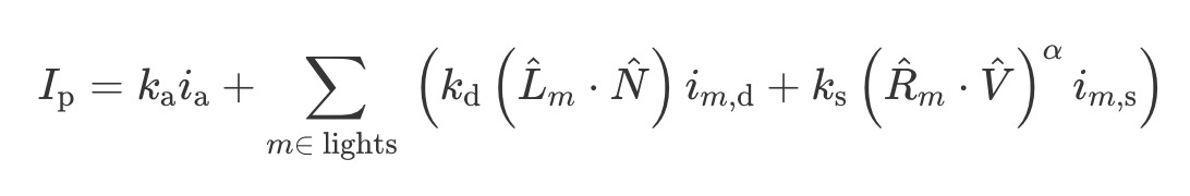
公式里的
根据上面的公式,我们把多个光照的计算结果相加,就能得到光照下几何体的最终颜色了。
不过,这里的 Phong 反射模型实际上是真实物理世界光照的简化模型,因为它只考虑光源的光作用于物体,没有考虑各个物体之间的反射光。所以我们最终实现出的效果也只是自然界效果的一种近似,不过这种近似也高度符合真实情况了。
在一般的图形库或者图形框架中,会提供符合 Phong 反射模型的物体材质,比如 ThreeJS 中,就支持各种光源和反射材质。
# 实现完整的 Phong 反射模型
Phong 反射模型的实现分为三步:定义光源模型、定义几何体材质和实现着色器。
# 1. 定义光源模型
环境光比较特殊,我们将它单独抽象出来,放在一个 ambientLight 的属性中,而其他的光源一共有 5 个属性与材质无关,如下表。
这样就可以定义一个 Phong 类。这个类由一个环境光属性和其他三种光源的集合组合而成,表示一个可以添加和删除光源的对象。它的主要作用是添加和删除光源,并把光源的属性通过 uniforms 访问器属性转换成对应的 uniform 变量。
class Phong {
  constructor(ambientLight = [0.5, 0.5, 0.5]) {
    this.ambientLight = ambientLight;
    this.directionalLights = new Set();
    this.pointLights = new Set();
    this.spotLights = new Set();
  }

  addLight(light) {
    const {position, direction, color, decay, angle} = light;
    if(!position && !direction) throw new TypeError('invalid light');
    light.color = color || [1, 1, 1];
    if(!position) this.directionalLights.add(light);
    else {
      light.decay = decay || [0, 0, 1];
      if(!angle) {
        this.pointLights.add(light);
      } else {
        this.spotLights.add(light);
      }
    }
  }

  removeLight(light) {
    if(this.directionalLights.has(light)) this.directionalLights.delete(light);
    else if(this.pointLights.has(light)) this.pointLights.delete(light);
    else if(this.spotLights.has(light)) this.spotLights.delete(light);
  }

  get uniforms() {
    const MAX_LIGHT_COUNT = 16; // 最多每种光源设置 16 个
    this._lightData = this._lightData || {};
    const lightData = this._lightData;

    lightData.directionalLightDirection = lightData.directionalLightDirection || {value: new Float32Array(MAX_LIGHT_COUNT * 3)};
    lightData.directionalLightColor = lightData.directionalLightColor || {value: new Float32Array(MAX_LIGHT_COUNT * 3)};

    lightData.pointLightPosition = lightData.pointLightPosition || {value: new Float32Array(MAX_LIGHT_COUNT * 3)};
    lightData.pointLightColor = lightData.pointLightColor || {value: new Float32Array(MAX_LIGHT_COUNT * 3)};
    lightData.pointLightDecay = lightData.pointLightDecay || {value: new Float32Array(MAX_LIGHT_COUNT * 3)};

    lightData.spotLightDirection = lightData.spotLightDirection || {value: new Float32Array(MAX_LIGHT_COUNT * 3)};
    lightData.spotLightPosition = lightData.spotLightPosition || {value: new Float32Array(MAX_LIGHT_COUNT * 3)};
    lightData.spotLightColor = lightData.spotLightColor || {value: new Float32Array(MAX_LIGHT_COUNT * 3)};
    lightData.spotLightDecay = lightData.spotLightDecay || {value: new Float32Array(MAX_LIGHT_COUNT * 3)};
    lightData.spotLightAngle = lightData.spotLightAngle || {value: new Float32Array(MAX_LIGHT_COUNT)};

    [...this.directionalLights].forEach((light, idx) => {
      lightData.directionalLightDirection.value.set(light.direction, idx * 3);
      lightData.directionalLightColor.value.set(light.color, idx * 3);
    });

    [...this.pointLights].forEach((light, idx) => {
      lightData.pointLightPosition.value.set(light.position, idx * 3);
      lightData.pointLightColor.value.set(light.color, idx * 3);
      lightData.pointLightDecay.value.set(light.decay, idx * 3);
    });

    [...this.spotLights].forEach((light, idx) => {
      lightData.spotLightPosition.value.set(light.position, idx * 3);
      lightData.spotLightColor.value.set(light.color, idx * 3);
      lightData.spotLightDecay.value.set(light.decay, idx * 3);
      lightData.spotLightDirection.value.set(light.direction, idx * 3);
      lightData.spotLightAngle.value[idx] = light.angle;
    });

    return {
      ambientLight: {value: this.ambientLight},
      ...lightData,
    };
  }
}
2
3
4
5
6
7
8
9
10
11
12
13
14
15
16
17
18
19
20
21
22
23
24
25
26
27
28
29
30
31
32
33
34
35
36
37
38
39
40
41
42
43
44
45
46
47
48
49
50
51
52
53
54
55
56
57
58
59
60
61
62
63
64
65
66
67
68
69
70
71
72
有了这个类之后,我们就可以创建并添加各种光源了。比如下面的代码添加了一个平行光和两个点光源。
const phong = new Phong();

// 添加一个平行光
phong.addLight({
  direction: [-1, 0, 0],
});

// 添加两个点光源
phong.addLight({
  position: [-3, 3, 0],
  color: [1, 0, 0],
});
phong.addLight({
  position: [3, 3, 0],
  color: [0, 0, 1],
});
2
3
4
5
6
7
8
9
10
11
12
13
14
15
16
# 2. 定义几何体材质
几何体材质决定了光反射的性质。
与材质有关的变量有 3 个,分别是 matrialReflection (材质反射率)、specularFactor (镜面反射强度)、以及 shininess (镜面反射光洁度)。
我们可以创建一个 Matrial 类,来定义物体的材质。与光源类相比,这个类非常简单,只是设置这三个参数,并通过 uniforms 访问器属性,获得它的 uniform 数据结构形式。
class Material {
  constructor(reflection, specularFactor = 0, shininess = 50) {
    this.reflection = reflection;
    this.specularFactor = specularFactor;
    this.shininess = shininess;
  }

  get uniforms() {
    return {
      materialReflection: {value: this.reflection},
      specularFactor: {value: this.specularFactor},
      shininess: {value: this.shininess},
    };
  }
}
2
3
4
5
6
7
8
9
10
11
12
13
14
15
接着,我们就可以创建 matrial 对象了。下面一共创建 4 个 matrial 对象,分别对应要显示的四个几何体的材质。
const matrial1 = new Material(new Color('#0000ff'), 2.0);
const matrial2 = new Material(new Color('#ff00ff'), 2.0);
const matrial3 = new Material(new Color('#008000'), 2.0);
const matrial4 = new Material(new Color('#ff0000'), 2.0);
2
3
4
有了 phong 对象和 matrial 对象,我们就可以给几何体创建 WebGL 程序了。我们就使用上面四个 WebGL 程序,来创建真正的几何体网格,并将它们渲染出来。
const program1 = new Program(gl, {
  vertex,
  fragment,
  uniforms: {
    ...matrial1.uniforms,
    ...phong.uniforms,
  },
});
const program2 = new Program(gl, {
  vertex,
  fragment,
  uniforms: {
    ...matrial2.uniforms,
    ...phong.uniforms,
  },
});
const program3 = new Program(gl, {
  vertex,
  fragment,
  uniforms: {
    ...matrial3.uniforms,
    ...phong.uniforms,
  },
});
const program4 = new Program(gl, {
  vertex,
  fragment,
  uniforms: {
    ...matrial4.uniforms,
    ...phong.uniforms,
  },
});
2
3
4
5
6
7
8
9
10
11
12
13
14
15
16
17
18
19
20
21
22
23
24
25
26
27
28
29
30
31
32
# 3. 实现着色器
着色器的代码实现比较复杂。
首先,我们来看光照相关的 uniform 变量的声明。这里,我们声明了 vec3 和 float 数组,数组的大小为 16。这样,对于每一种光源,我们都可以支持 16 个。
#define MAX_LIGHT_COUNT 16
uniform mat4 viewMatrix;

uniform vec3 ambientLight;
uniform vec3 directionalLightDirection[MAX_LIGHT_COUNT];
uniform vec3 directionalLightColor[MAX_LIGHT_COUNT];
uniform vec3 pointLightColor[MAX_LIGHT_COUNT];
uniform vec3 pointLightPosition[MAX_LIGHT_COUNT];
uniform vec3 pointLightDecay[MAX_LIGHT_COUNT];
uniform vec3 spotLightColor[MAX_LIGHT_COUNT];
uniform vec3 spotLightDirection[MAX_LIGHT_COUNT];
uniform vec3 spotLightPosition[MAX_LIGHT_COUNT];
uniform vec3 spotLightDecay[MAX_LIGHT_COUNT];
uniform float spotLightAngle[MAX_LIGHT_COUNT];

uniform vec3 materialReflection;
uniform float shininess;
uniform float specularFactor;
2
3
4
5
6
7
8
9
10
11
12
13
14
15
16
17
18
接下来实现计算 phong 反射模型的主体逻辑。事实上,处理平行光、点光源、聚光灯的主体逻辑类似,都是循环处理每个光源,再计算入射光方向,然后计算漫反射以及镜面反射,最终将结果返回。
float getSpecular(vec3 dir, vec3 normal, vec3 eye) {
  vec3 reflectionLight = reflect(-dir, normal);
  float eyeCos = max(dot(eye, reflectionLight), 0.0);
  return specularFactor *  pow(eyeCos, shininess);
}

vec4 phongReflection(vec3 pos, vec3 normal, vec3 eye) {
  float specular = 0.0;
  vec3 diffuse = vec3(0);

  // 处理平行光
  for(int i = 0; i < MAX_LIGHT_COUNT; i++) {
    vec3 dir = directionalLightDirection[i];
    if(dir.x == 0.0 && dir.y == 0.0 && dir.z == 0.0) continue;
    vec4 d = viewMatrix * vec4(dir, 0.0);
    dir = normalize(-d.xyz);
    float cos = max(dot(dir, normal), 0.0);
    diffuse += cos * directionalLightColor[i];
    specular += getSpecular(dir, normal, eye);
  }

  // 处理点光源
  for(int i = 0; i < MAX_LIGHT_COUNT; i++) {
    vec3 decay = pointLightDecay[i];
    if(decay.x == 0.0 && decay.y == 0.0 && decay.z == 0.0) continue;
    vec3 dir = (viewMatrix * vec4(pointLightPosition[i], 1.0)).xyz - pos;
    float dis = length(dir);
    dir = normalize(dir);
    float cos = max(dot(dir, normal), 0.0);
    float d = min(1.0, 1.0 / (decay.x * pow(dis, 2.0) + decay.y * dis + decay.z));
    diffuse += d * cos * pointLightColor[i];
    specular += getSpecular(dir, normal, eye);
  }

  // 处理聚光灯
  for(int i = 0; i < MAX_LIGHT_COUNT; i++) {
    vec3 decay = spotLightDecay[i];
    if(decay.x == 0.0 && decay.y == 0.0 && decay.z == 0.0) continue;

    vec3 dir = (viewMatrix * vec4(spotLightPosition[i], 1.0)).xyz - pos;
    float dis = length(dir);
    dir = normalize(dir);

    // 聚光灯的朝向
    vec3 spotDir = (viewMatrix * vec4(spotLightDirection[i], 0.0)).xyz;
    // 通过余弦值判断夹角范围
    float ang = cos(spotLightAngle[i]);
    float r = step(ang, dot(dir, normalize(-spotDir)));

    float cos = max(dot(dir, normal), 0.0);
    float d = min(1.0, 1.0 / (decay.x * pow(dis, 2.0) + decay.y * dis + decay.z));
    diffuse += r * d * cos * spotLightColor[i];
    specular += r * getSpecular(dir, normal, eye);
  }

  return vec4(diffuse, specular);
}
2
3
4
5
6
7
8
9
10
11
12
13
14
15
16
17
18
19
20
21
22
23
24
25
26
27
28
29
30
31
32
33
34
35
36
37
38
39
40
41
42
43
44
45
46
47
48
49
50
51
52
53
54
55
56
57
最后在 main 函数中,调用 phongReflection 函数来合成颜色。
void main() {
  vec3 eyeDirection = normalize(vCameraPos - vPos);
  vec4 phong = phongReflection(vPos, vNormal, eyeDirection);

  // 合成颜色
  gl_FragColor.rgb = phong.w + (phong.xyz + ambientLight) * materialReflection;
  gl_FragColor.a = 1.0;
}
2
3
4
5
6
7
8
最终呈现的视觉效果如下,也可以看这里 (opens new window)。可以发现,因为我们一共设置了 3 个光源,一个平行光、两个点光源,它们都能够产生镜面反射。所以,这些光源叠加在一起后,这个球体就呈现出 3 个镜面高光。
# Phong 反射模型的局限性
虽然,phong 反射模型已经比较接近于真实的物理模型,不过它仍然是真实模型的一种近似。因为它没有考虑物体反射光对其他物体的影响,也没有考虑物体对光线遮挡产生的阴影。
当然,我们可以完善这个模型。比如,将物体本身反射光(主要是镜面反射光)对其他物体的影响纳入到模型中。另外,我们也要考虑物体的阴影。当我们把这些因素更多地考虑进去的时候,我们的模型就会更加接近真实世界的物理模型。
当我们渲染 3D 图形的时候,要呈现越接近真实的效果,往往要考虑更多的参数,因此所需的计算量也越大,那我们就需要有更强的渲染能力,比如,更好的显卡,更快的 CPU 和 GPU,并且也需要我们尽可能地优化计算的性能。但是,有很多时候,我们需要在细节和性能上做出平衡和取舍。
# 如何用法线贴图模拟真实物体表面
在真实世界中,大部分物体的表面都是凹凸不平的,只有处理好物体凹凸表面的光照效果,我们才能更加真实地模拟物体表面。在图形学中就有一种对应的技术,叫做法线贴图。
# 使用法线贴图给几何体表面增加凹凸效果
首先,我们用 Phong 反射模型绘制一个灰色的立方体,并给它添加两道平行光。
import {Phong, Material, vertex as v, fragment as f} from '../common/lib/phong.js';

const scene = new Transform();

const phong = new Phong();
phong.addLight({
  direction: [0, -3, -3],
});
phong.addLight({
  direction: [0, 3, 3],
});
const matrial = new Material(new Color('#808080'));

const program = new Program(gl, {
  vertex: v,
  fragment: f,
  uniforms: {
    ...phong.uniforms,
    ...matrial.uniforms,
  },
});

const geometry = new Box(gl);
const cube = new Mesh(gl, {geometry, program});
cube.setParent(scene);
cube.rotation.x = -Math.PI / 2;
2
3
4
5
6
7
8
9
10
11
12
13
14
15
16
17
18
19
20
21
22
23
24
25
26
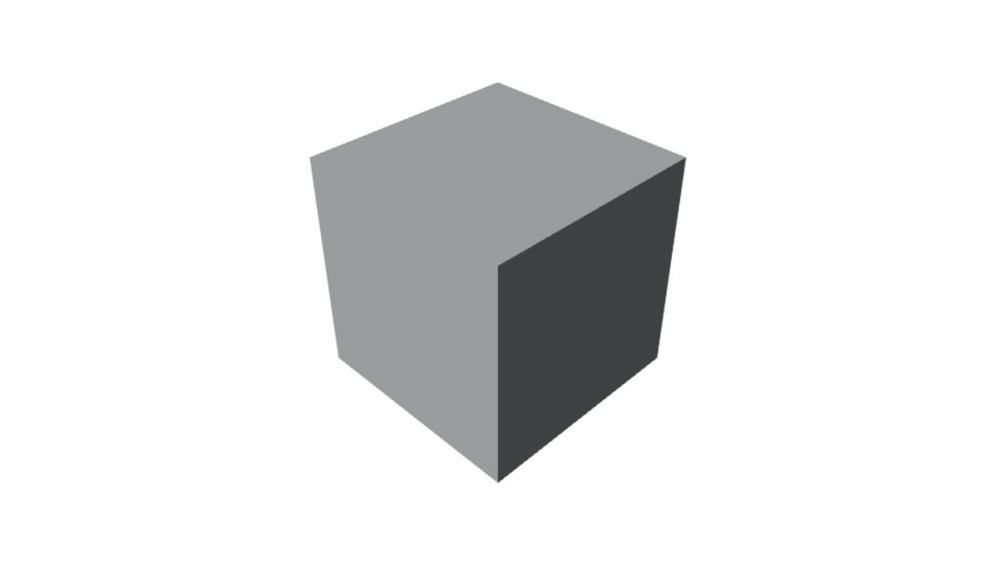
现在这个立方体的表面是光滑的,如果我们想在立方体的表面贴上凹凸的花纹。我们可以加载一张法线纹理,这是一张偏蓝色调的纹理图片。
const normalMap = await loadTexture('../assets/normal_map.png');
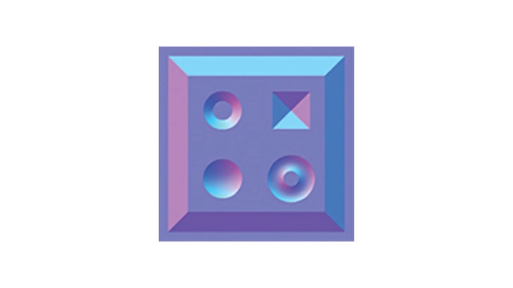
为什么这张纹理图片是偏蓝色调的呢?实际上,这张纹理图片保存的是几何体表面的每个像素的法向量数据。
正常情况下,光滑立方体每个面的法向量是固定的,但如果表面有凹凸的花纹,那不同位置的法向量就会发生变化。在切线空间中,因为法线都偏向于 z 轴,也就是法向量偏向于 (0,0,1),所以转换成的法线纹理就偏向于蓝色。如果我们根据花纹将每个点的法向量都保存下来,就会得到上面那张法线纹理的图片。
# 切线空间
切线空间(Tangent Space)是一个特殊的坐标系,它是由几何体顶点所在平面的 uv 坐标和法线构成的。
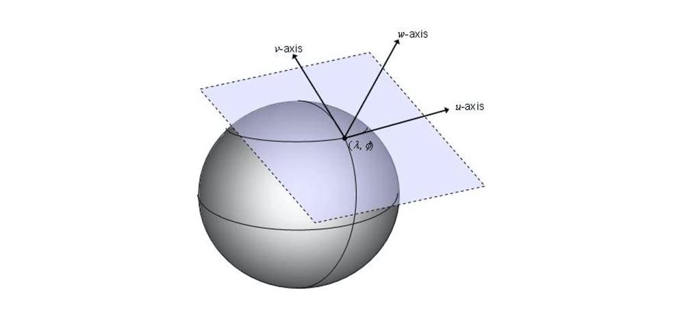
切线空间的三个轴,一般用 T (Tangent)、B (Bitangent)、N (Normal) 三个字母表示,所以切线空间也被称为 TBN 空间。其中 T 表示切线、B 表示副切线、N 表示法线。
对于大部分三维几何体来说,因为每个点的法线不同,所以它们各自的切线空间也不同。
# 切线空间中的 TBN 如何计算
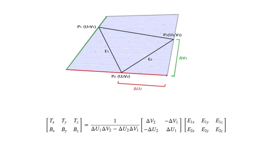
首先回忆下如何计算几何体三角形网格的法向量。假设一个三角形网格有三个点 v1、v2、v3,我们把边 v1v2 记为 e1,边 v1v3 记为 e2,那三角形的法向量就是 e1 和 e2 的叉积表示的归一化向量。
function getNormal(v1, v2, v3) {
  const e1 = Vec3.sub(v2, v1);
  const e2 = Vec3.sub(v3, v1);
  const normal = Vec3.cross(e1, e1).normalize();
  return normal;
}
2
3
4
5
6
# 计算切线和副切线
而计算切线和副切线,要比计算法线复杂得多,不过,因为数学推导过程 (opens new window)比较复杂,我们只要记住结论就可以了。
// 先进行向量计算,然后将 tang 和 bitang 的值添加到 geometry 对象中去
function createTB(geometry) {
  const {position, index, uv} = geometry.attributes;
  if(!uv) throw new Error('NO uv.');
  function getTBNTriangle(p1, p2, p3, uv1, uv2, uv3) {
    const edge1 = new Vec3().sub(p2, p1);
    const edge2 = new Vec3().sub(p3, p1);
    const deltaUV1 = new Vec2().sub(uv2, uv1);
    const deltaUV2 = new Vec2().sub(uv3, uv1);

    const tang = new Vec3();
    const bitang = new Vec3();

    const f = 1.0 / (deltaUV1.x * deltaUV2.y - deltaUV2.x * deltaUV1.y);

    tang.x = f * (deltaUV2.y * edge1.x - deltaUV1.y * edge2.x);
    tang.y = f * (deltaUV2.y * edge1.y - deltaUV1.y * edge2.y);
    tang.z = f * (deltaUV2.y * edge1.z - deltaUV1.y * edge2.z);

    tang.normalize();

    bitang.x = f * (-deltaUV2.x * edge1.x + deltaUV1.x * edge2.x);
    bitang.y = f * (-deltaUV2.x * edge1.y + deltaUV1.x * edge2.y);
    bitang.z = f * (-deltaUV2.x * edge1.z + deltaUV1.x * edge2.z);

    bitang.normalize();

    return {tang, bitang};
  }

  const size = position.size;
  if(size < 3) throw new Error('Error dimension.');

  const len = position.data.length / size;
  const tang = new Float32Array(len * 3);
  const bitang = new Float32Array(len * 3);

  for(let i = 0; i < index.data.length; i += 3) {
    const i1 = index.data[i];
    const i2 = index.data[i + 1];
    const i3 = index.data[i + 2];

    const p1 = [position.data[i1 * size], position.data[i1 * size + 1], position.data[i1 * size + 2]];
    const p2 = [position.data[i2 * size], position.data[i2 * size + 1], position.data[i2 * size + 2]];
    const p3 = [position.data[i3 * size], position.data[i3 * size + 1], position.data[i3 * size + 2]];

    const u1 = [uv.data[i1 * 2], uv.data[i1 * 2 + 1]];
    const u2 = [uv.data[i2 * 2], uv.data[i2 * 2 + 1]];
    const u3 = [uv.data[i3 * 2], uv.data[i3 * 2 + 1]];

    const {tang: t, bitang: b} = getTBNTriangle(p1, p2, p3, u1, u2, u3);
    tang.set(t, i1 * 3);
    tang.set(t, i2 * 3);
    tang.set(t, i3 * 3);
    bitang.set(b, i1 * 3);
    bitang.set(b, i2 * 3);
    bitang.set(b, i3 * 3);
  }
  geometry.addAttribute('tang', {data: tang, size: 3});
  geometry.addAttribute('bitang', {data: bitang, size: 3});
  return geometry;
}
2
3
4
5
6
7
8
9
10
11
12
13
14
15
16
17
18
19
20
21
22
23
24
25
26
27
28
29
30
31
32
33
34
35
36
37
38
39
40
41
42
43
44
45
46
47
48
49
50
51
52
53
54
55
56
57
58
59
60
61
62
# 构建 TBN 矩阵来计算法向量
有了 tang 和 bitang 之后,我们就可以构建 TBN 矩阵来计算法线了。
这里的 TBN 矩阵的作用,就是将法线贴图里面读取的法向量数据,转换为对应的切线空间中实际的法向量。这里的切线空间,实际上对应着我们观察者(相机)位置的坐标系。
接下来根据顶点着色器和片元着色器来说说怎么构建 TBN 矩阵得出法线方向。
先看顶点着色器,我们增加了 tang 和 bitang 这两个属性。注意,这里我们用了 webgl2.0 的写法,因为 WebGL2.0 对应 OpenGL ES3.0,所以这段代码和我们之前看到的着色器代码略有不同。
#version 300 es // 表示这段代码是 OpenGL ES3.0 的
precision highp float;

in vec3 position; // in 对应变量的输入,取代 WebGL2.0 的 attribute
in vec3 normal;
in vec2 uv;
in vec3 tang;
in vec3 bitang;

uniform mat4 modelMatrix;
uniform mat4 modelViewMatrix;
uniform mat4 viewMatrix;
uniform mat4 projectionMatrix;
uniform mat3 normalMatrix;
uniform vec3 cameraPosition;

out vec3 vNormal; // out 对应变量的输出,取代 WebGL2.0 的 varying
out vec3 vPos;
out vec2 vUv;
out vec3 vCameraPos;
out mat3 vTBN;

void main() {
  vec4 pos = modelViewMatrix * vec4(position, 1.0);
  vPos = pos.xyz;
  vUv = uv;
  vCameraPos = (viewMatrix * vec4(cameraPosition, 1.0)).xyz;
  // 因为 normal、tang 和 bitang 都需要换到世界坐标中,
  // 所以我们要记得将它们左乘法向量矩阵 normalMatrix
  vNormal = normalize(normalMatrix * normal);

  vec3 N = vNormal;
  vec3 T = normalize(normalMatrix * tang);
  vec3 B = normalize(normalMatrix * bitang);

  vTBN = mat3(T, B, N); // 构建 TBN 矩阵

  gl_Position = projectionMatrix * pos;
}
2
3
4
5
6
7
8
9
10
11
12
13
14
15
16
17
18
19
20
21
22
23
24
25
26
27
28
29
30
31
32
33
34
35
36
37
38
39
接下来是片元着色器的代码。这里面从法线纹理中提取数据和 TBN 矩阵来计算对应的法线的方法就是,把法线纹理贴图中提取的数据转换到 [-1,1] 区间,然后左乘 TBN 矩阵并归一化。
#version 300 es
precision highp float;

#define MAX_LIGHT_COUNT 16
uniform mat4 viewMatrix;

uniform vec3 ambientLight;
uniform vec3 directionalLightDirection[MAX_LIGHT_COUNT];
uniform vec3 directionalLightColor[MAX_LIGHT_COUNT];
uniform vec3 pointLightColor[MAX_LIGHT_COUNT];
uniform vec3 pointLightPosition[MAX_LIGHT_COUNT];
uniform vec3 pointLightDecay[MAX_LIGHT_COUNT];
uniform vec3 spotLightColor[MAX_LIGHT_COUNT];
uniform vec3 spotLightDirection[MAX_LIGHT_COUNT];
uniform vec3 spotLightPosition[MAX_LIGHT_COUNT];
uniform vec3 spotLightDecay[MAX_LIGHT_COUNT];
uniform float spotLightAngle[MAX_LIGHT_COUNT];

uniform vec3 materialReflection;
uniform float shininess;
uniform float specularFactor;

uniform sampler2D tNormal;

in vec3 vNormal;
in vec3 vPos;
in vec2 vUv;
in vec3 vCameraPos;
in mat3 vTBN;

out vec4 FragColor;

float getSpecular(vec3 dir, vec3 normal, vec3 eye) {
  vec3 reflectionLight = reflect(-dir, normal);
  float eyeCos = max(dot(eye, reflectionLight), 0.0);
  return specularFactor *  pow(eyeCos, shininess);
}

vec4 phongReflection(vec3 pos, vec3 normal, vec3 eye) {
  float specular = 0.0;
  vec3 diffuse = vec3(0);

  // 处理平行光
  for(int i = 0; i < MAX_LIGHT_COUNT; i++) {
    vec3 dir = directionalLightDirection[i];
    if(dir.x == 0.0 && dir.y == 0.0 && dir.z == 0.0) continue;
    vec4 d = viewMatrix * vec4(dir, 0.0);
    dir = normalize(-d.xyz);
    float cos = max(dot(dir, normal), 0.0);
    diffuse += cos * directionalLightColor[i];
    specular += getSpecular(dir, normal, eye);
  }

  // 处理点光源
  for(int i = 0; i < MAX_LIGHT_COUNT; i++) {
    vec3 decay = pointLightDecay[i];
    if(decay.x == 0.0 && decay.y == 0.0 && decay.z == 0.0) continue;
    vec3 dir = (viewMatrix * vec4(pointLightPosition[i], 1.0)).xyz - pos;
    float dis = length(dir);
    dir = normalize(dir);
    float cos = max(dot(dir, normal), 0.0);
    float d = min(1.0, 1.0 / (decay.x * pow(dis, 2.0) + decay.y * dis + decay.z));
    diffuse += d * cos * pointLightColor[i];
    specular += getSpecular(dir, normal, eye);
  }

  // 处理聚光灯
  for(int i = 0; i < MAX_LIGHT_COUNT; i++) {
    vec3 decay = spotLightDecay[i];
    if(decay.x == 0.0 && decay.y == 0.0 && decay.z == 0.0) continue;

    vec3 dir = (viewMatrix * vec4(spotLightPosition[i], 1.0)).xyz - pos;
    float dis = length(dir);
    dir = normalize(dir);

    // 聚光灯的朝向
    vec3 spotDir = (viewMatrix * vec4(spotLightDirection[i], 0.0)).xyz;
    // 通过余弦值判断夹角范围
    float ang = cos(spotLightAngle[i]);
    float r = step(ang, dot(dir, normalize(-spotDir)));

    float cos = max(dot(dir, normal), 0.0);
    float d = min(1.0, 1.0 / (decay.x * pow(dis, 2.0) + decay.y * dis + decay.z));
    diffuse += r * d * cos * spotLightColor[i];
    specular += r * getSpecular(dir, normal, eye);
  }

  return vec4(diffuse, specular);
}

vec3 getNormal() {
  vec3 n = texture(tNormal, vUv).rgb * 2.0 - 1.0;
  return normalize(vTBN * n);
}

void main() {
  vec3 eyeDirection = normalize(vCameraPos - vPos);
  vec3 normal = getNormal();
  vec4 phong = phongReflection(vPos, normal, eyeDirection);

  // 合成颜色
  FragColor.rgb = phong.w + (phong.xyz + ambientLight) * materialReflection;
  FragColor.a = 1.0;
}
2
3
4
5
6
7
8
9
10
11
12
13
14
15
16
17
18
19
20
21
22
23
24
25
26
27
28
29
30
31
32
33
34
35
36
37
38
39
40
41
42
43
44
45
46
47
48
49
50
51
52
53
54
55
56
57
58
59
60
61
62
63
64
65
66
67
68
69
70
71
72
73
74
75
76
77
78
79
80
81
82
83
84
85
86
87
88
89
90
91
92
93
94
95
96
97
98
99
100
101
102
103
104
然后,我们将经过处理之后的法向量传给 phongReflection 计算光照,就得到了法线贴图后的结果,效果如下,也可以看这里 (opens new window)。
# 使用偏导数来实现法线贴图
构建 TBN 矩阵求法向量的方法有点麻烦。事实上,还有一种更巧妙的方法,不需要用顶点数据计算几何体的切线和副切线,而是直接用坐标插值和法线纹理来计算。
vec3 getNormal() {
  vec3 pos_dx = dFdx(vPos.xyz);
  vec3 pos_dy = dFdy(vPos.xyz);
  vec2 tex_dx = dFdx(vUv);
  vec2 tex_dy = dFdy(vUv);

  vec3 t = normalize(pos_dx * tex_dy.t - pos_dy * tex_dx.t);
  vec3 b = normalize(-pos_dx * tex_dy.s + pos_dy * tex_dx.s);
  mat3 tbn = mat3(t, b, normalize(vNormal));

  vec3 n = texture(tNormal, vUv).rgb * 2.0 - 1.0;
  return normalize(tbn * n);
}
2
3
4
5
6
7
8
9
10
11
12
13
这段代码中,dFdx、dFdy 是 GLSL 内置函数,可以求插值的属性在 x、y 轴上的偏导数。
为什么要求偏导数呢?
偏导数其实就代表插值的属性向量在 x、y 轴上的变化率,或者说曲面的切线。然后,我们再将顶点坐标曲面切线与 uv 坐标的切线求叉积,就能得到垂直于两条切线的法线。
我们在 x、y 两个方向上求出的两条法线,就对应 TBN 空间的切线 tang 和副切线 bitang。然后,我们使用偏导数构建 TBN 矩阵,同样也是把 TBN 矩阵左乘从法线纹理中提取出的值,就可以计算出对应的法向量了。
这样做的好处是,我们不需要预先计算几何体的 tang 和 bitang 了。不过在片元着色器中计算偏导数也有一定的性能开销,所以各有利弊,我们可以根据不同情况选择不同的方案。
# 法线贴图的应用
法线贴图除了给几何体表面增加花纹以外,还可以用来增强物体细节,让物体看起来更加真实。比如,实现一个石块被变化的光源照亮效果 (opens new window)。
对应的片元着色器核心代码如下:
uniform float uTime;

void main() {
  vec3 eyeDirection = normalize(vCameraPos - vPos);
  vec3 normal = getNormal();
  vec4 phong = phongReflection(vPos, normal, eyeDirection);
  // vec4 phong = phongReflection(vPos, vNormal, eyeDirection);

  vec3 tex = texture(tMap, vUv).rgb;
  vec3 light = normalize(vec3(sin(uTime), 1.0, cos(uTime)));
  float shading = dot(normal, light) * 0.5;

  FragColor.rgb = tex + shading;
  FragColor.a = 1.0;
}
2
3
4
5
6
7
8
9
10
11
12
13
14
15
# 法线贴图总结
法线贴图是用一张图片来存储表面的法线数据。这张图片叫做法线纹理,它上面的每个像素对应一个坐标点的法线数据。
要想使用法线纹理的数据,我们还需要构建 TBN 矩阵。这个矩阵通过向量、矩阵乘法将法线数据转换到世界坐标中。
构建 TBN 矩阵我们有两个方法:
一个是根据几何体顶点数据来计算切线(Tangent)、副切线(Bitangent),然后结合法向量一起构建 TBN 矩阵。
另一个方法是使用偏导数来计算,这样我们就不用预先在顶点中计算 Tangent 和 Bitangent 了。
两种方法各有利弊,我们可以根据实际情况来合理选择。
# 如何绘制带宽度的曲线
在可视化应用中,我们经常需要绘制一些带有特定宽度的曲线。比如说,在地理信息可视化中,我们会使用曲线来描绘路径,而在 3D 地球可视化中,我们会使用曲线来描述飞线、轮廓线等等。
# 连线方式和线帽形状
曲线是由线段连接而成的,两个线段中间转折的部分,就是 lineJoin。如果线宽只有一个像素,那么连接处没有什么不同的形式,就是直接连接。但如果线宽超过一个像素,那么连接处的缺口,就会有不同的填充方式,而这些不同的填充方式,就对应了不同的 lineJoin。
下面的图就展示了四种不同的 lineJoin。其中,miter 是尖角,round 是圆角,bevel 是斜角,none 是不添加 lineJoin。
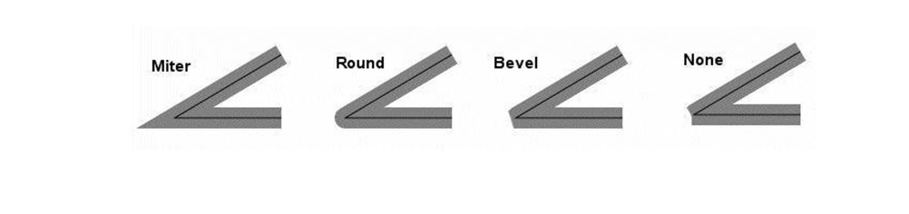
而 lineCap 就是指曲线头尾部的形状,它有三种类型。第一种是 square,方形线帽,它会在线段的头尾端延长线宽的一半。第二种 round 也叫圆弧线帽,它会在头尾端延长一个半圆。第三种是 butt,就是不添加线帽。

# 用 Canvas2D 绘制带宽度的曲线
在 Canvas2D 中,要绘制带宽度的曲线非常简单,我们直接通过 API 设置上下文对象的 lineWidth (opens new window) 即可。而且,Canvas2D 还支持不同的 lineJoin (opens new window)、lineCap (opens new window) 设置以及 miterLimit (opens new window) 设置。
接下来就在 Canvas2D 的上下文中,通过设置 lineJoin 和 lineCap 属性,来实现不同的曲线效果。
绘制的代码如下,最终效果看这里 (opens new window)。
function drawPolyline(context, points, {lineWidth = 1, lineJoin = 'miter', lineCap = 'butt', miterLimit = 10} = {}) {
  context.lineWidth = lineWidth;
  context.lineJoin = lineJoin;
  context.lineCap = lineCap;
  context.miterLimit = miterLimit;
  context.beginPath();
  context.moveTo(...points[0]);
  for (let i = 1; i < points.length; i++) {
    context.lineTo(...points[i]);
  }
  context.stroke();
}

const canvas = document.querySelector('canvas');
const ctx = canvas.getContext('2d');
const points = [
  [100, 100],
  [100, 200],
  [200, 150],
  [300, 200],
  [300, 100],
];
ctx.strokeStyle = 'red';
drawPolyline(ctx, points, {lineWidth: 10, lineCap: 'round', lineJoin: 'miter', miterLimit: 1.5});
ctx.strokeStyle = 'blue';
drawPolyline(ctx, points);
2
3
4
5
6
7
8
9
10
11
12
13
14
15
16
17
18
19
20
21
22
23
24
25
26
# 用 WebGL 绘制带宽度的曲线
在 WebGL 中,绘制带宽度的曲线非常麻烦,因为没有现成的 API 可以使用,是一个难点。
这个时候,我们可以使用挤压曲线的技术来得到带宽度的曲线,挤压曲线的具体步骤可以总结为三步:
确定端点和转角的挤压方向,端点可以沿线段的法线挤压,转角则通过两条线段延长线的单位向量求和的方式获得。
确定端点和转角挤压的长度,端点两个方向的挤压长度是线宽 lineWidth 的一半。求转角挤压长度的时候,我们要先计算方向向量和线段法线的余弦,然后将线宽 lineWidth 的一半除以我们计算出的余弦值。
由步骤 1、2 计算出顶点后,我们构建三角网格化的几何体顶点数据,然后将 Geometry 对象返回。
这样,我们就可以用 WebGL 绘制出有宽度的曲线了。
下面具体介绍下绘制过程。
我们先从绘制宽度为 1 的曲线开始。因为 WebGL 本身就支持线段类的图元,所以我们直接用图元就能绘制出宽度为 1 的曲线。
与 Canvas2D 类似,我们直接设置 position 顶点坐标,然后设置 mode 为 gl.LINE_STRIP。这里的 LINE_STRIP 是一种图元类型,表示以首尾连接的线段方式绘制。这样,我们就可以得到宽度为 1 的折线了。
import {Renderer, Program, Geometry, Transform, Mesh} from '../common/lib/ogl/index.mjs';

const vertex = `
  attribute vec2 position;

  void main() {
    gl_PointSize = 10.0;
    float scale = 1.0 / 256.0;
    mat3 projectionMatrix = mat3(
      scale, 0, 0,
      0, -scale, 0,
      -1, 1, 1
    );
    vec3 pos = projectionMatrix * vec3(position, 1);
    gl_Position = vec4(pos.xy, 0, 1);
  }
`;


const fragment = `
  precision highp float;
  void main() {
    gl_FragColor = vec4(1, 0, 0, 1);
  }
`;

const canvas = document.querySelector('canvas');
const renderer = new Renderer({
  canvas,
  width: 512,
  height: 512,
});

const gl = renderer.gl;
gl.clearColor(1, 1, 1, 1);


const program = new Program(gl, {
  vertex,
  fragment,
});

const geometry = new Geometry(gl, {
position: {size: 2,
  data: new Float32Array(
    [
      100, 100,
      100, 200,
      200, 150,
      300, 200,
      300, 100,
    ],
  )},
});

const scene = new Transform();
const polyline = new Mesh(gl, {geometry, program, mode: gl.LINE_STRIP});
polyline.setParent(scene);

renderer.render({scene});
2
3
4
5
6
7
8
9
10
11
12
13
14
15
16
17
18
19
20
21
22
23
24
25
26
27
28
29
30
31
32
33
34
35
36
37
38
39
40
41
42
43
44
45
46
47
48
49
50
51
52
53
54
55
56
57
58
59
60
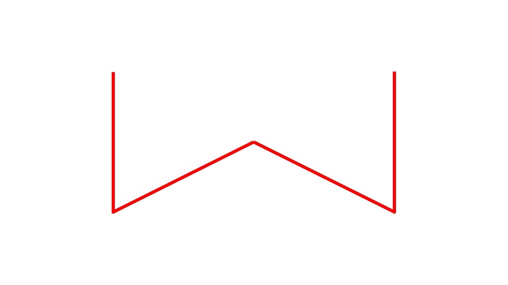
# 挤压曲线
我们可以用一种挤压(Extrude)曲线的技术,通过将曲线的顶点沿法线方向向两侧移出,让 1 个像素的曲线变宽。
如上图所示,黑色折线是原始的 1 个像素宽度的折线,蓝色虚线组成的是我们最终要生成的带宽度曲线,红色虚线是顶点移动的方向。
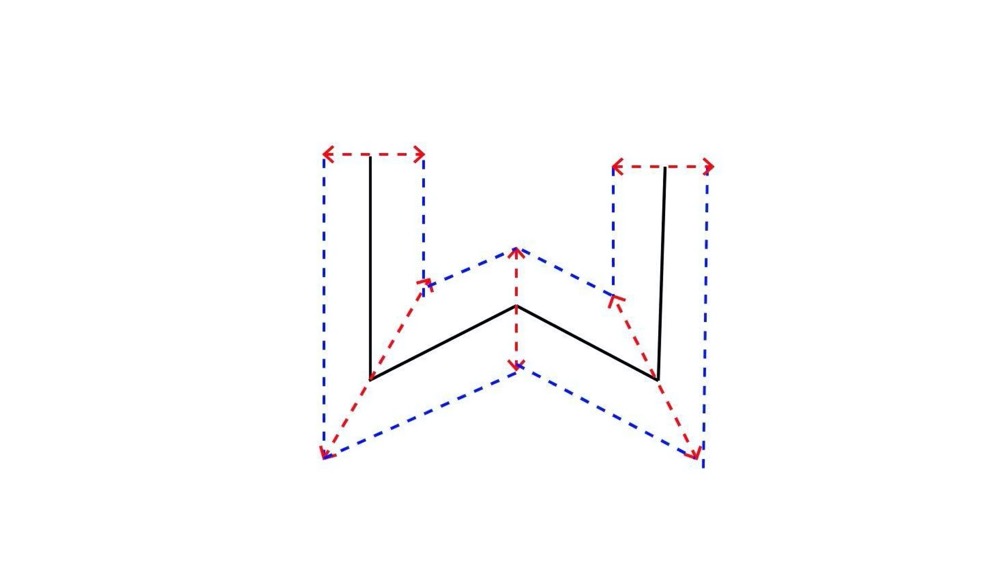
# 确定挤压方向
因为折线两个端点的挤压只和一条线段的方向有关,而转角处顶点的挤压和相邻两条线段的方向都有关,所以顶点移动的方向,我们要分两种情况讨论。
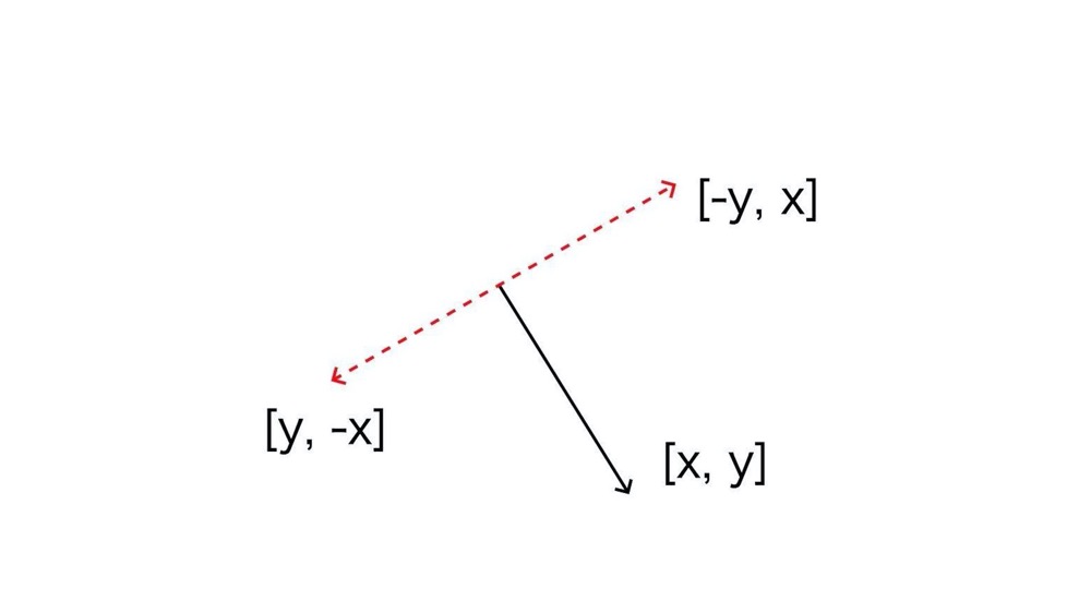
首先,是折线的端点。假设线段的向量为(x, y),因为它移动方向和线段方向垂直,所以我们只要沿法线方向移动它就可以了。根据垂直向量的点积为 0,我们很容易得出顶点的两个移动方向为(-y, x)和(y, -x)。如下图所示:
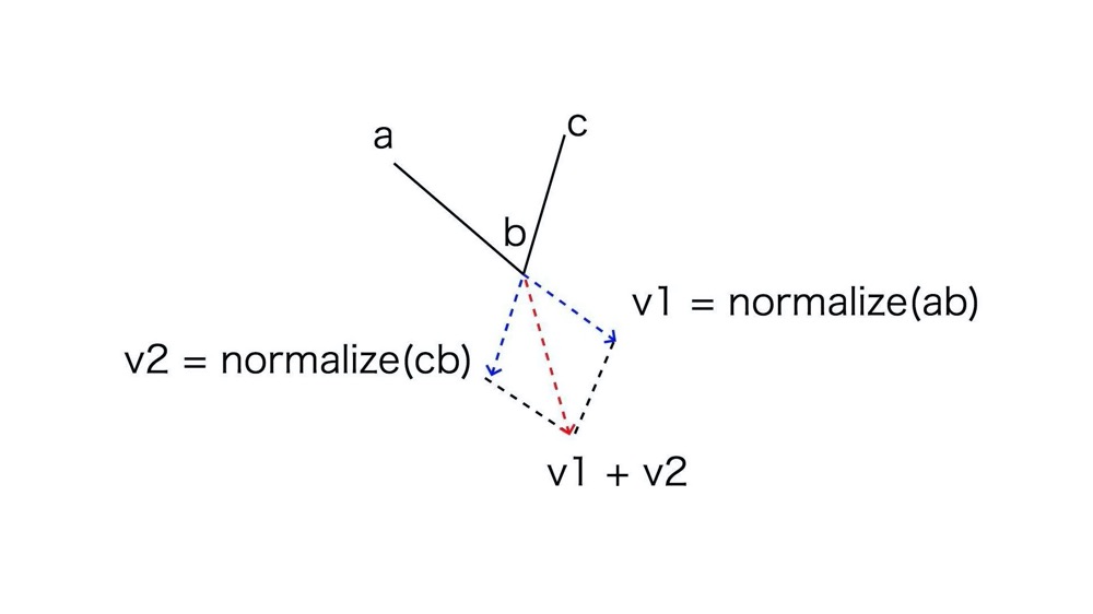
接下来再确定转角的挤压方向,假设有折线 abc,b 是转角。我们延长 ab,就能得到一个单位向量 v1,反向延长 bc,可以得到另一个单位向量 v2,那么挤压方向就是向量 v1+v2 的方向,以及相反的 -(v1+v2) 的方向。如下图所示:
# 确定挤压长度
得到了挤压方向之后,接下来就需要确定挤压向量的长度。
首先是折线端点的挤压长度,它等于 lineWidth 的一半。而转角的挤压长度就比较复杂了,需要计算一下。
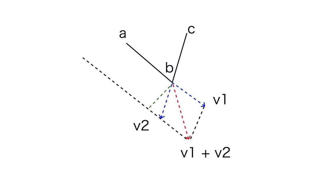
如上图所示,绿色这条辅助线应该等于 lineWidth 的一半,而它又恰好是 v1+v2 在绿色这条向量方向的投影,所以,我们可以先用向量点积求出红色虚线和绿色虚线夹角的余弦值,然后用 lineWidth 的一半除以这个值,得到的就是挤压向量的长度了。具体代码实现如下:
function extrudePolyline(gl, points, {thickness = 10} = {}) {
  const halfThick = 0.5 * thickness;
  const innerSide = []; // 存储向内挤压的点
  const outerSide = []; // 存储向外挤压的点

  // 构建挤压顶点
  for(let i = 1; i < points.length - 1; i++) {
    const v1 = (new Vec2()).sub(points[i], points[i - 1]).normalize(); // v1、v2 是线段的延长线
    const v2 = (new Vec2()).sub(points[i], points[i + 1]).normalize();
    const v = (new Vec2()).add(v1, v2).normalize(); // 得到挤压方向
    const norm = new Vec2(-v1.y, v1.x); // 法线方向
    const cos = norm.dot(v); // 计算法线方向与挤压方向的余弦值
    const len = halfThick / cos; // 算出挤压长度
    if(i === 1) { // 起始点
      const v0 = new Vec2(...norm).scale(halfThick);
      outerSide.push((new Vec2()).add(points[0], v0));
      innerSide.push((new Vec2()).sub(points[0], v0));
    }
    v.scale(len);
    outerSide.push((new Vec2()).add(points[i], v));
    innerSide.push((new Vec2()).sub(points[i], v));
    if(i === points.length - 2) { // 结束点
      const norm2 = new Vec2(v2.y, -v2.x);
      const v0 = new Vec2(...norm2).scale(halfThick);
      outerSide.push((new Vec2()).add(points[points.length - 1], v0));
      innerSide.push((new Vec2()).sub(points[points.length - 1], v0));
    }
  }
  // ...
}
2
3
4
5
6
7
8
9
10
11
12
13
14
15
16
17
18
19
20
21
22
23
24
25
26
27
28
29
30
# 构建 Geometry 对象
补充 extrudePolyline 函数的后半部分,根据 innerSide 和 outerSide 中的顶点来构建三角网格化的几何体顶点数据,最终返回 Geometry 对象。
function extrudePolyline(gl, points, {thickness = 10} = {}) {
  // ...
  const count = innerSide.length * 4 - 4;
  const position = new Float32Array(count * 2);
  const index = new Uint16Array(6 * count / 4);

  // 创建 geometry 对象
  for(let i = 0; i < innerSide.length - 1; i++) {
    const a = innerSide[i],
      b = outerSide[i],
      c = innerSide[i + 1],
      d = outerSide[i + 1];

    const offset = i * 4;
    index.set([offset, offset + 1, offset + 2, offset + 2, offset + 1, offset + 3], i * 6);
    position.set([...a, ...b, ...c, ...d], i * 8);
  }

  return new Geometry(gl, {
    position: {size: 2, data: position},
    index: {data: index},
  });
}
2
3
4
5
6
7
8
9
10
11
12
13
14
15
16
17
18
19
20
21
22
23
24
构建出来的折线的顶点数据如下图:
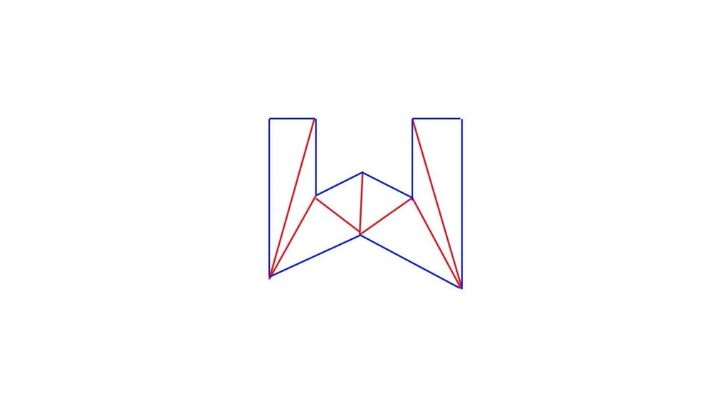
最后,只要调用 extrudePolyline,传入折线顶点和宽度,然后用返回的 Geometry 对象来构建三角网格对象,将它渲染出来就可以了。最终效果看这里 (opens new window)。
const geometry = extrudePolyline(gl, points, {lineWidth: 10});

const scene = new Transform();
const polyline = new Mesh(gl, {geometry, program});
polyline.setParent(scene);

renderer.render({scene});
2
3
4
5
6
7
这样,我们就在 WebGL 中实现了与 Canvas2D 一样带宽度的曲线。
不过,这里我们只实现了最基础的带宽度曲线,它对应于 Canvas2D 中的 lineJoin 为 miter,lineCap 为 butt 的曲线。我们也可以基于 extrudePolyline 函数,对它进行扩展,实现 lineJoins 为 bevel 或 round,lineCap 为 square 或 round 的曲线。基本原理是一样的,只要计算出相应属性下对应的顶点就行了。
# 绘制 Github 贡献 3D 图表
# 第一步:准备要展现的数据
GitHub 上有第三方 API 可以获得指定用户的 GitHub 贡献数据,具体可以看 Github Contributions API (opens new window) 这个项目。
通过 API,我们可以事先保存好一份 JSON 格式的数据,具体的格式和内容大致如下:
// github_contributions_akira-cn.json
{
  "contributions": [
    {
      "date": "2020-06-12",
      "count": 1, // 每一天的提交次数
      "color":"#c6e48b", // 颜色数据
    },
    // ...
  ],
}
2
3
4
5
6
7
8
9
10
11
这份 JSON 文件的数据很多,所以我们可以写一个函数,根据传入的时间对数据进行过滤。
let cache = null;
async function getData(toDate = new Date()) {
  if(!cache) {
    const data = await (await fetch('../assets/github_contributions_akira-cn.json')).json();
    cache = data.contributions.map((o) => {
      o.date = new Date(o.date.replace(/-/g, '/'));
      return o;
    });
  }
  // 要拿到 toData 日期之前大约一年的数据(52 周)
  let start = 0,
    end = cache.length;
  // 用二分法查找
  while(start < end - 1) {
    const mid = Math.floor(0.5 * (start + end));
    const {date} = cache[mid];
    if(date <= toDate) end = mid;
    else start = mid;
  }
  // 获得对应的一年左右的数据
  let day;
  if(end >= cache.length) {
    day = toDate.getDay();
  } else {
    const lastItem = cache[end];
    day = lastItem.date.getDay();
  }
  // 根据当前星期几,再往前拿 52 周的数据
  const len = 7 * 52 + day + 1;
  const ret = cache.slice(end, end + len);
  if(ret.length < len) {
    // 日期超过了数据范围,补齐数据
    const pad = new Array(len - ret.length).fill({count: 0, color: '#ebedf0'});
    ret.push(...pad);
  }
  return ret;
}
2
3
4
5
6
7
8
9
10
11
12
13
14
15
16
17
18
19
20
21
22
23
24
25
26
27
28
29
30
31
32
33
34
35
36
37
# 第二步:用 SpriteJS 渲染数据、完成绘图
SpriteJS (opens new window) 是一个支持树状元素结构的渲染库。也就是说,它和我们前端操作 DOM 类似,通过将元素一一添加到渲染树上,就可以完成最终的渲染。
SpriteJS 的 3D 部分是基于 OGL 库实现的,它在 OGL 的基础上,对几何体元素进行了类似 DOM 元素的封装。这样我们创建几何体元素就可以像操作 DOM 一样方便了,直接用 d3 库的 selection 子模块来操作就可以了。
# 1. 创建 Scene 对象
像 DOM 有 documentElement 作为根元素一样,SpriteJS 也有根元素。
SpriteJS 的根元素是一个 Scene 对象,对应一个 DOM 元素作为容器。更形象点来说,我们可以把 Scene 理解为一个 “场景”。那 SpriteJS 中渲染图形,都要在这个 “场景” 中进行。
创建 Scene 对象需要两个参数。
一个参数是 container,它是一个 HTML 元素,在这里是一个 id 为 stage 的元素,这个元素会作为 SpriteJS 的容器元素,之后 SpriteJS 会在这个元素上创建 Canvas 子元素。
第二个参数是 displayRatio,这个参数是用来设置显示分辨率的。在 Canvas 绘图那里提到过,为了让绘制出来的图形能够适配不同的显示设备,我们要把 Canvas 的像素宽高和 CSS 样式宽高设置成不同的值。所以这里,我们把 displayRatio 设为 2,就可以让像素宽高是 CSS 样式宽高的 2 倍,对于一些像素密度为 2 的设备(如 iPhone 的屏幕),这么设置才不会让画布上绘制的图片、文字变得模糊。
const container = document.getElementById('stage');

const scene = new Scene({
  container,
  displayRatio: 2,
});
2
3
4
5
6
# 2. 创建 Layer 对象
有了 scene 对象,我们再创建一个或多个 Layer 对象,也可以理解为是一个或者多个 “图层”。
在 SpriteJS 中,一个 Layer 对象就对应于一个 Canvas 画布。
// 把相机的视角设置为 35 度,坐标位置为(2, 6, 9),相机朝向坐标原点。
const layer = scene.layer3d('fglayer', {
  camera: {
    fov: 35,
  },
});
layer.camera.attributes.pos = [2, 6, 9];
layer.camera.lookAt([0, 0, 0]);
2
3
4
5
6
7
8
# 3. 将数据转换成柱状元素
接着,我们就要把数据转换成画布上的长方体元素。这里可以借助 d3-selection (opens new window) 这个库,d3 是一个数据驱动文档的模型,d3-selection 能够通过数据操作文档树,添加元素节点。
不过,在使用 d3-selection 添加元素前,我们要先创建用来 3D 展示的 WebGL 程序。
因为 SpriteJS 提供了一些预置的着色器,比如 shaders.GEOMETRY 着色器,就是默认支持 phong 反射模型的一组着色器,我们直接调用它就可以了。
const program = layer.createProgram({
  vertex: shaders.GEOMETRY.vertex,
  fragment: shaders.GEOMETRY.fragment,
});
2
3
4
创建好 WebGL 程序之后,我们就可以获取数据,用数据来操作文档树了。
const dataset = await getData();
const max = d3.max(dataset, (a) => {
  return a.count;
});

/* globals d3 */
const selection = d3.select(layer);
// 遍历数据,创建元素节点
const chart = selection.selectAll('cube')
  .data(dataset)
  .enter()
  .append(() => {
    // 创建 Cube 元素,即长方体
    // dataset 的每一条记录对应一个 Cube 元素
    return new Cube(program);
  })
  // 设置每个 Cube 元素的样式
  .attr('width', 0.14) // 长
  .attr('depth', 0.14) // 宽
  .attr('height', 1) // 高
  .attr('scaleY', (d) => { // y 轴的缩放
    // 这里的 max 是指一年的提交记录中,提交代码最多那天的数值
    // 这样,我们就可以保证 scaleY 的值在 0~1 之间,既不会太小、也不会太大
    // 这种用相对数值来做可视化展现的做法,是可视化处理数据的一种常用基础技巧
    return d.count / max;
  })
  .attr('pos', (d, i) => { // 位置坐标,根据数据的索引设置 x 和 z 来决定
    const x0 = -3.8 + 0.0717 + 0.0015;
    const z0 = -0.5 + 0.05 + 0.0015;
    const x = x0 + 0.143 * Math.floor(i / 7);
    const z = z0 + 0.143 * (i % 7);
    // 由于 Cube 的坐标基于中心点对齐的,现在想让它们变成底部对齐,就需要把 y 设置为 d.count/max 的一半
    return [x, 0.5 * d.count /max, z];
  })
  .attr('colors', (d, i) => { // 长方体的颜色
    return d.color;
  });
2
3
4
5
6
7
8
9
10
11
12
13
14
15
16
17
18
19
20
21
22
23
24
25
26
27
28
29
30
31
32
33
34
35
36
37
到这,就实现了一个基本的 3D 效果了。
# 第三步:补充细节,实现更好的视觉效果
# 1. 增加光照
可以给这个柱状图增加一些视觉上的细节效果,比如添加光照。这里修改了环境光,把颜色设置成 (0.5, 0.5, 0.5, 1),再添加一道白色的平行光,方向是 (-3, -3, -1)。这样的话,柱状图就会有光照效果了。
const layer = scene.layer3d('fglayer', {
  ambientColor: [0.5, 0.5, 0.5, 1],
  camera: {
    fov: 35,
  },
});
layer.camera.attributes.pos = [2, 6, 9];
layer.camera.lookAt([0, 0, 0]);

const light = new Light({
  direction: [-3, -3, -1],
  color: [1, 1, 1, 1],
});

layer.addLight(light);
2
3
4
5
6
7
8
9
10
11
12
13
14
15
# 2. 增加底座
除此之外,我们还可以给柱状图增加一个底座。
const fragment = `
  precision highp float;
  precision highp int;
  varying vec4 vColor;
  varying vec2 vUv;
  void main() {
    float x = fract(vUv.x * 53.0);
    float y = fract(vUv.y * 7.0);
    x = smoothstep(0.0, 0.1, x) - smoothstep(0.9, 1.0, x);
    y = smoothstep(0.0, 0.1, y) - smoothstep(0.9, 1.0, y);
    gl_FragColor = vColor * (x + y);
  }
`;

const axisProgram = layer.createProgram({
  vertex: shaders.TEXTURE.vertex,
  fragment,
});

const ground = new Cube(axisProgram, {
  width: 7.6,
  height: 0.1,
  y: -0.049, // not 0.05 to avoid z-fighting
  depth: 1,
  colors: 'rgba(0, 0, 0, 0.1)',
});

layer.append(ground);
2
3
4
5
6
7
8
9
10
11
12
13
14
15
16
17
18
19
20
21
22
23
24
25
26
27
28
# z-fighting 问题
在上面的代码中,我们将底座的高度设置为 0.1,y 的值本来应该是 -0.1 的一半,也就是 -0.05,但是我们设置为了 -0.049。少了 0.001 是为了让上层的柱状图稍微 “嵌入” 到底座里,从而避免因为底座上部和柱状图底部的 z 坐标一样,导致渲染的时候由于次序问题出现闪烁,这个问题在图形学术语里面有一个名字叫做 z-fighting。
z-fighting 是 3D 绘图中的一个常见问题。
在 WebGL 中绘制 3D 物体,一般我们开启了深度检测之后,引擎会自动计算 3D 物体的深度,让离观察者很近的物体面,把离观察者比较远和背对着观察者的物体面遮挡住。
那具体是怎么遮挡的呢?
其实是根据物体在相机空间中的 z 坐标来判断的。
但有一种特殊情况,就是两个面的 z 坐标相同,又有重叠的部分。这时候,引擎就可能一会儿先渲染 A 面,过一会儿又先去渲染 B 面,这样渲染出来的内容就出现了 “闪烁” 现象,这就是 z-fighting。
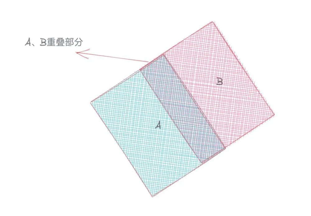
z-fighting 有很多解决方法,比如可以人为指定一下几何体渲染的次序,或者让它们的坐标不要完全相同。这里采用的就是第二种方法。
# 3. 增加动画
为了让实现出来的图形更有趣,我们再增加一个过渡动画,让柱状图的高度从不显示,到慢慢显示出来。最终效果也可以看这里 (opens new window)。
const chart = selection.selectAll('cube')
  .data(dataset)
  .enter()
  .append(() => {
    return new Cube(program);
  })
  .attr('width', 0.14)
  .attr('depth', 0.14)
  .attr('height', 1)
  .attr('scaleY', 0.001) // 把 scaleY 直接设为 0.001
  .attr('pos', (d, i) => {
    const x0 = -3.8 + 0.0717 + 0.0015;
    const z0 = -0.5 + 0.05 + 0.0015;
    const x = x0 + 0.143 * Math.floor(i / 7);
    const z = z0 + 0.143 * (i % 7);
    return [x, 0, z];
  })
  .attr('colors', (d, i) => {
    return d.color;
  });
2
3
4
5
6
7
8
9
10
11
12
13
14
15
16
17
18
19
20
// 用 d3.scaleLinear 来创建一个线性的缩放过程
const linear = d3.scaleLinear()
  .domain([0, max])
  .range([0, 1.0]);

// 再通过 chart.trainsition 来实现这个线性动画
chart.transition()
  .duration(2000)
  .attr('scaleY', (d, i) => {
    return linear(d.count);
  })
  .attr('y', (d, i) => {
    return 0.5 * linear(d.count);
  });
2
3
4
5
6
7
8
9
10
11
12
13
14